Compute Reference Force with Constant Drive

This example computes the reference muscle force using constant descending drive. This force is used as the target for optimizing the oscillating drive DC offset in Phase 3.

Note

Purpose: Establish force baseline using Watanabe network parameters

• 800 motor neurons

• 400 descending drive neurons

• 30% connectivity

• Constant drive frequency (configurable, default 40 Hz)

• Poisson process (order 1)

Configuration: Adjust DD_DRIVE_HZ at the top of the script (default: 40 Hz)

Output: Reference force saved to results/watanabe_optimization/force_reference.json

MyoGen Components Used:

• AlphaMN__Pool: Pool of 800 alpha motor neurons with exponentially distributed recruitment thresholds. Each neuron is a biophysically detailed NEURON model with soma, dendrites, and ion channels.

• DescendingDrive__Pool: Pool of 400 “descending drive” neurons that generate Poisson spike trains. These represent cortical/brainstem input to motor neurons. poisson_batch_size=1 creates order-1 (renewal) Poisson processes.

• Network: Container that manages populations and synaptic connections between them. Supports probabilistic connectivity (connect()) and external input (connect_from_external()).

• RecruitmentThresholds: Generates recruitment threshold distribution following Fuglevand/DeLuca models. The mode="combined" blends exponential and linear distributions.

• ForceModel: Converts motor neuron spike trains to muscle force using Fuglevand’s twitch model. Each motor unit has amplitude and contraction time determined by recruitment threshold.

Workflow Position: Step 1 of 6 - Run this first to establish baseline force.

Next Step: Run 02_optimize_oscillating_dc.py to find DC offset for Phase 3.

Import Libraries

import json
import os

os.environ["MPLBACKEND"] = "Agg"
if "DISPLAY" in os.environ:
    del os.environ["DISPLAY"]

import warnings
from pathlib import Path

import matplotlib.pyplot as plt
import numpy as np
import quantities as pq
from neo import Block, Segment, SpikeTrain
from neuron import h

from myogen import RANDOM_GENERATOR
from myogen.simulator import RecruitmentThresholds
from myogen.simulator.core.force.force_model import ForceModel
from myogen.simulator import Network
from myogen.simulator.neuron.populations import AlphaMN__Pool, DescendingDrive__Pool
from myogen.utils.helper import calculate_firing_rate_statistics
from myogen.utils.nmodl import load_nmodl_mechanisms

warnings.filterwarnings("ignore")
plt.style.use("fivethirtyeight")

USER CONFIGURATION - Adjust these parameters as needed

# Constant descending drive frequency (Hz)
# This is the baseline drive for Phase 1 (constant stimulation)
# - Watanabe original: 65 Hz
# - Lower values (e.g., 40 Hz): lower force output, fewer recruited units
# - Higher values (e.g., 80 Hz): higher force output, more recruited units
DD_DRIVE_HZ = 40.0

Define Simulation Parameters

# Watanabe network parameters (original specification)
N_MOTOR_UNITS = 800  # Watanabe specification
N_DD_NEURONS = 400  # Watanabe specification
DD_CONNECTIVITY = 0.3  # Watanabe specification (30%)
SYNAPTIC_WEIGHT = 0.05  # DD→MN synaptic weight (µS)

# Simulation parameters
SIMULATION_TIME_MS = 10000.0  # 10 seconds for steady-state force
TIMESTEP_MS = 0.1  # Integration timestep (ms)

# Force scaling (convert normalized force to Newtons)
MAX_FORCE_N = 100.0  # Maximum voluntary contraction force (N) - typical for finger flexors

# File paths - Watanabe-specific directory
try:
    _script_dir = Path(__file__).parent
except NameError:
    _script_dir = Path.cwd()
RESULTS_DIR = _script_dir / "results" / "watanabe_optimization"
RESULTS_DIR.mkdir(exist_ok=True, parents=True)

print(f"\nComputing Reference Force with {DD_DRIVE_HZ:.1f} Hz Constant Drive (Watanabe Network)")
print("=" * 60)
print(f"Motor neurons: {N_MOTOR_UNITS}")
print(f"DD neurons: {N_DD_NEURONS}")
print(f"Connection probability: {DD_CONNECTIVITY:.1%}")
print(f"Drive frequency: {DD_DRIVE_HZ:.1f} Hz (constant)")
print("Process type: Poisson (batch size: 1)")
print("=" * 60 + "\n")

Computing Reference Force with 40.0 Hz Constant Drive (Watanabe Network)
============================================================
Motor neurons: 800
DD neurons: 400
Connection probability: 30.0%
Drive frequency: 40.0 Hz (constant)
Process type: Poisson (batch size: 1)
============================================================

Load NEURON Mechanisms and Setup Network

MyoGen uses NEURON as its simulation engine. Before creating any neurons, we must load the compiled NMODL mechanisms (ion channels, synapses, etc.).

load_nmodl_mechanisms()
h.secondorder = 2  # Crank-Nicolson integration (2nd order accurate, stable)

# Create recruitment thresholds for 800 neurons
# ---------------------------------------------
# Recruitment thresholds determine:
#   1. Which motor units activate first (low threshold = low force, recruited early)
#   2. Motor unit properties (twitch amplitude, contraction time)
#
# Parameters:
#   - recruitment_range__ratio=100: Largest MU has 100x threshold of smallest
#   - mode="combined": Blends Fuglevand exponential + DeLuca linear distributions
#   - deluca__slope: Controls steepness of threshold curve
recruitment_thresholds, _ = RecruitmentThresholds(
    N=N_MOTOR_UNITS,
    recruitment_range__ratio=100,
    deluca__slope=5,
    konstantin__max_threshold__ratio=1.0,
    mode="combined",
)

# Create motor neuron pool
# ------------------------
# AlphaMN__Pool creates N biophysically detailed motor neurons.
# Each neuron has:
#   - Soma with Hodgkin-Huxley-style channels
#   - Dendrites for synaptic input
#   - Properties scaled by recruitment threshold (input resistance, rheobase)
#
# The config_file specifies morphology and channel parameters.
motor_neuron_pool = AlphaMN__Pool(
    recruitment_thresholds__array=recruitment_thresholds,
    config_file="alpha_mn_default.yaml",
)

# Create descending drive pool with Poisson process (Watanabe)
# ------------------------------------------------------------
# DescendingDrive__Pool creates "virtual" neurons that generate spike trains
# at a specified rate. They don't have membrane dynamics - just Poisson processes.
#
# Parameters:
#   - process_type="poisson": Renewal Poisson process
#   - poisson_batch_size=1: Order-1 (memoryless) - Watanabe specification
#     Higher values create more regular spike trains (order-k gamma process)
descending_drive_pool = DescendingDrive__Pool(
    n=N_DD_NEURONS,
    timestep__ms=TIMESTEP_MS * pq.ms,
    process_type="poisson",
    poisson_batch_size=1,  # Order 1 Poisson (Watanabe specification)
)

Build Network

The Network class manages populations and connections between them. It handles the complexity of creating synapses in NEURON.

network = Network({"DD": descending_drive_pool, "aMN": motor_neuron_pool})

# Connect DD → aMN with 30% probability (Watanabe specification)
# --------------------------------------------------------------
# This creates SHARED input: multiple motor neurons receive spikes from
# the same DD neurons, creating correlated activity across the pool.
#
# With probability=0.3, each motor neuron connects to ~30% of DD neurons
# (~120 connections), while each DD neuron projects to ~30% of motor neurons.
network.connect(
    source="DD",
    target="aMN",
    probability=DD_CONNECTIVITY,
    weight__uS=SYNAPTIC_WEIGHT * pq.uS,
)

# External input to DD population
# --------------------------------
# Creates NetCon objects that allow us to deliver events to DD neurons.
# In the simulation loop, we'll use these to trigger spikes based on
# the drive signal.
network.connect_from_external(source="cortical_input", target="DD", weight__uS=1.0 * pq.uS)
dd_netcons = network.get_netcons("cortical_input", "DD")

Setup Spike Recording

mn_spike_recorders = []
for cell in motor_neuron_pool:
    spike_recorder = h.Vector()
    nc = h.NetCon(cell.soma(0.5)._ref_v, None, sec=cell.soma)
    nc.threshold = 50
    nc.record(spike_recorder)
    mn_spike_recorders.append(spike_recorder)

Generate Drive Signal (65 Hz constant)

time_points = int(SIMULATION_TIME_MS / TIMESTEP_MS)
drive_signal = np.ones(time_points) * DD_DRIVE_HZ + np.clip(
    RANDOM_GENERATOR.normal(0, 1.0, size=time_points), 0, None
)

Run Simulation

h.load_file("stdrun.hoc")
h.dt = TIMESTEP_MS
h.tstop = SIMULATION_TIME_MS

# Initialize voltages
for section, voltage in zip(*motor_neuron_pool.get_initialization_data()):
    section.v = voltage
for section, voltage in zip(*descending_drive_pool.get_initialization_data()):
    section.v = voltage

h.finitialize()

print("Running simulation...")
step_counter = 0
while h.t < h.tstop:
    current_drive = drive_signal[min(step_counter, len(drive_signal) - 1)]
    for dd_cell in descending_drive_pool:
        if dd_cell.integrate(current_drive):
            if h.t < h.tstop:
                dd_netcons[dd_cell.pool__ID].event(h.t + 1)
    h.fadvance()
    step_counter += 1

print("Simulation complete!\n")

Running simulation...
Simulation complete!

Process Spike Trains

dt_s = h.dt / 1000.0
mn_segment = Segment(name="Motor Neurons")
mn_segment.spiketrains = [
    SpikeTrain(
        recorder.as_numpy() / 1000 * pq.s,
        t_stop=SIMULATION_TIME_MS / 1000 * pq.s,
        sampling_rate=(1 / dt_s * (pq.Hz)),
        sampling_period=dt_s * pq.s,
        name=f"MN_{i}",
    )
    for i, recorder in enumerate(mn_spike_recorders)
]

spike_train__Block = Block(name="Motor Unit Pool")
spike_train__Block.segments = [mn_segment]

Calculate Firing Rate Statistics

stats = calculate_firing_rate_statistics(mn_segment.spiketrains)
fr_mean = float(stats["FR_mean"])
fr_std = float(stats["FR_std"])
n_active = int(stats["n_active"])

print("Firing Rate Statistics:")
print(f"  Active units: {n_active}/{N_MOTOR_UNITS} ({n_active / N_MOTOR_UNITS * 100:.1f}%)")
print(f"  Mean firing rate: {fr_mean:.2f} Hz")
print(f"  Std deviation: {fr_std:.2f} Hz")
print(f"  Coefficient of variation: {fr_std / fr_mean:.3f}\n")

Firing Rate Statistics:
  Active units: 377/800 (47.1%)
  Mean firing rate: 5.80 Hz
  Std deviation: 2.69 Hz
  Coefficient of variation: 0.464

Generate Force Output

The ForceModel implements Fuglevand’s motor unit twitch model:

• Each motor unit produces a twitch waveform: F(t) = P * (t/T) * exp(1 - t/T)

• P (peak force) and T (contraction time) depend on recruitment threshold

• Low-threshold units: small P, short T → small, fast twitches

• High-threshold units: large P, long T → large, slow twitches

The force model convolves each unit’s twitch with its spike train, then sums across all units to get total muscle force.

force_model = ForceModel(
    recruitment_thresholds=recruitment_thresholds,
    recording_frequency__Hz=2048 * pq.Hz,  # Output sampling rate
    longest_duration_rise_time__ms=90.0 * pq.ms,  # Slowest unit's rise time
    contraction_time_range_factor=3,  # Ratio of slowest/fastest T
)

# Generate force from spike trains
# Returns a NEO AnalogSignal with units of "arbitrary" (sum of normalized twitches)
force_output = force_model.generate_force(spike_train__Block=spike_train__Block)
force_raw = force_output.magnitude[:, 0]  # Arbitrary units (sum of MU twitches)
force_time = force_output.times.rescale(pq.s).magnitude

# Normalize force to 0-1 range, then scale to Newtons
# (ForceModel outputs sum of MU twitch forces, not normalized values)
force_max_raw = np.max(force_raw)
force_signal = (force_raw / force_max_raw) * MAX_FORCE_N  # Scale to Newtons

Pool 1 Twitch trains (Numba):   0%|          | 0/800 [00:00<?, ?MU/s]
Pool 1 Twitch trains (Numba):   0%|          | 1/800 [00:00<01:35,  8.39MU/s]
Pool 1 Twitch trains (Numba): 100%|██████████| 800/800 [00:00<00:00, 4061.21MU/s]

Analyze Force Characteristics

# Use last 50% to avoid transients
steady_idx = len(force_signal) // 2
force_steady = force_signal[steady_idx:]

force_mean = np.mean(force_steady)
force_std = np.std(force_steady)
force_cov = force_std / force_mean

print(f"Reference Force Statistics ({DD_DRIVE_HZ:.1f} Hz constant drive):")
print(f"  Mean force: {force_mean:.2f} N")
print(f"  Std deviation: {force_std:.2f} N")
print(f"  Coefficient of variation: {force_cov:.3f}")
print(f"  Ripple amplitude: {(force_std / force_mean) * 100:.2f}%")
print(f"  Peak normalized force: {np.max(force_signal):.2f} N (= MAX_FORCE_N)\n")

Reference Force Statistics (40.0 Hz constant drive):
  Mean force: 67.29 N
  Std deviation: 10.14 N
  Coefficient of variation: 0.151
  Ripple amplitude: 15.07%
  Peak normalized force: 100.00 N (= MAX_FORCE_N)

Save Results

force_results = {
    "network_parameters": {
        "n_motor_units": N_MOTOR_UNITS,
        "dd_neurons": N_DD_NEURONS,
        "dd_connectivity": DD_CONNECTIVITY,
        "dd_drive__Hz": DD_DRIVE_HZ,
        "synaptic_weight__uS": SYNAPTIC_WEIGHT,
        "process_type": "poisson",
        "poisson_batch_size": 1,
    },
    "force_scaling": {
        "max_force__N": MAX_FORCE_N,
    },
    "firing_rate": {
        "mean__Hz": fr_mean,
        "std__Hz": fr_std,
        "n_active": n_active,
        "cov": fr_std / fr_mean,
    },
    "force": {
        "mean__N": force_mean,
        "std__N": force_std,
        "cov": force_cov,
        "ripple_percent": (force_std / force_mean) * 100,
    },
}

results_file = RESULTS_DIR / "force_reference.json"
with open(results_file, "w") as f:
    json.dump(force_results, f, indent=2)

print(f"Saved reference force results: {results_file}")
print(f"Reference drive: {DD_DRIVE_HZ:.1f} Hz constant")
print(f"\nNext step: Run 02_optimize_oscillating_dc.py to find DC offset for Phase 3")

Saved reference force results: /home/runner/work/MyoGen/MyoGen/examples/03_papers/watanabe/results/watanabe_optimization/force_reference.json
Reference drive: 40.0 Hz constant

Next step: Run 02_optimize_oscillating_dc.py to find DC offset for Phase 3

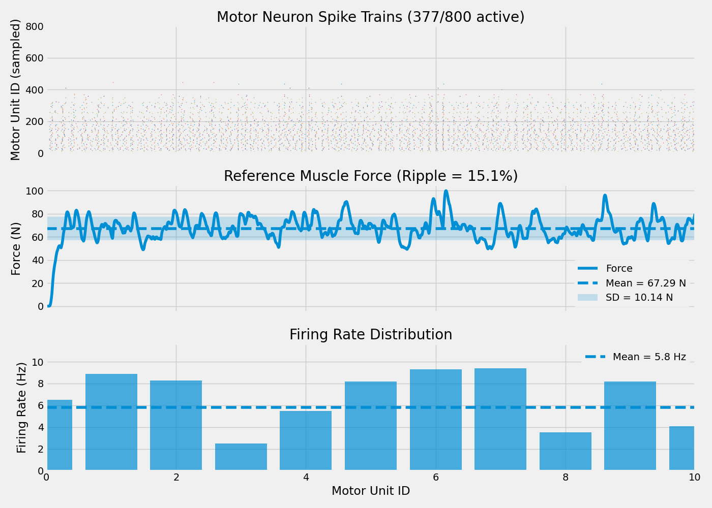
Visualize Results

fig, axes = plt.subplots(3, 1, figsize=(14, 10), sharex=True)

# 1. Motor neuron raster plot (sample every 5th neuron for visibility)
sample_interval = 5
for i, spiketrain in enumerate(mn_segment.spiketrains):
    if i % sample_interval == 0 and len(spiketrain) > 0:
        spike_times = spiketrain.rescale(pq.s).magnitude
        axes[0].scatter(spike_times, [i] * len(spike_times), s=0.5, alpha=0.6)

axes[0].set_ylabel("Motor Unit ID (sampled)")
axes[0].set_title(f"Motor Neuron Spike Trains ({n_active}/{N_MOTOR_UNITS} active)")
axes[0].set_ylim(-1, N_MOTOR_UNITS)

# 2. Force trace
axes[1].plot(force_time, force_signal, label="Force")
axes[1].axhline(force_mean, linestyle="--", label=f"Mean = {force_mean:.2f} N")
axes[1].fill_between(
    force_time,
    force_mean - force_std,
    force_mean + force_std,
    alpha=0.2,
    label=f"SD = {force_std:.2f} N",
)
axes[1].set_ylabel("Force (N)")
axes[1].set_title(f"Reference Muscle Force (Ripple = {force_cov * 100:.1f}%)")
axes[1].legend(framealpha=1.0, edgecolor="none")

# 3. Firing rate distribution
firing_rates = []
mu_ids = []
for i, st in enumerate(mn_segment.spiketrains):
    if len(st) > 2:
        rate = len(st) / (SIMULATION_TIME_MS / 1000.0)
        firing_rates.append(rate)
        mu_ids.append(i)

if firing_rates:
    axes[2].bar(mu_ids, firing_rates, alpha=0.7)
    axes[2].axhline(fr_mean, linestyle="--", label=f"Mean = {fr_mean:.1f} Hz")
    axes[2].set_xlabel("Motor Unit ID")
    axes[2].set_ylabel("Firing Rate (Hz)")
    axes[2].set_title("Firing Rate Distribution")
    axes[2].legend(framealpha=1.0, edgecolor="none")

for ax in axes:
    ax.set_xlim(0, SIMULATION_TIME_MS / 1000)

plt.tight_layout()
plt.savefig(RESULTS_DIR / "force_reference.png", dpi=150, bbox_inches="tight")
plt.show()