Surface Motor Unit Action Potentials

After having created the muscle model, we can simulate the surface EMG by creating a surface EMG model.

First step is to create MUAPs from the muscle model.

Note

The MUAPs are the action potentials of the motor units at the surface of the skin.

from pathlib import Path

import joblib
import matplotlib.pyplot as plt
import numpy as np
import quantities as pq

from myogen import simulator

plt.style.use("fivethirtyeight")

Define Parameters

The surface EMG is created using the SurfaceEMG object.

The SurfaceEMG object takes the following parameters:

• muscle_model: Muscle model

• sampling_frequency: Sampling frequency

• electrode_grid_dimensions: Electrode grid dimensions

• inter_electrode_distance: Inter-electrode distance

• fat_thickness: Fat thickness

• skin_thickness: Skin thickness

# Define simulation parameters
sampling_frequency = 2048.0 * pq.Hz

Load Muscle Model

Load muscle model from previous example

save_path = Path("./results")
muscle: simulator.Muscle = joblib.load(save_path / "muscle_model.pkl")

Create Surface EMG Model

The SurfaceEMG object is initialized with the muscle model, the electrode array, and the simulation parameters.

Note

For simplicity, we only simulate the first motor unit. This can be changed by modifying the MUs_to_simulate parameter.

This is to simulate the surface EMG from two different directions.

electrode_array_monopolar = simulator.SurfaceElectrodeArray(
    num_rows=5,
    num_cols=5,
    inter_electrode_distances__mm=5 * pq.mm,
    electrode_radius__mm=5 * pq.mm,
    differentiation_mode="monopolar",
    bending_radius__mm=muscle.radius__mm + muscle.skin_thickness__mm + muscle.fat_thickness__mm,
)

surface_emg = simulator.SurfaceEMG(
    muscle_model=muscle,
    electrode_arrays=[electrode_array_monopolar],
    sampling_frequency__Hz=sampling_frequency,
    sampling_points_in_t_and_z_domains=256,
    sampling_points_in_theta_domain=32,  # Restored to default (log-space Bessel implementation prevents overflow)
    MUs_to_simulate=[0, 1, 2, 3],  # Simulate MUs 0, 1, 2, and 3
    # iap_kernel_length__mm=None,  # Default: uses scaled fiber length (2.5× for boundary clearance)
    # The IAP kernel is automatically scaled to 2.5× the mean fiber length to:
    # 1. Prevent boundary truncation artifacts
    # 2. Allow full IAP wavefront development and decay
    # 3. Maintain proportionality to actual fiber lengths
    # Result: Realistic MUAP durations (8-10 ms) independent of sampling resolution N!
)

Simulate MUAPs

To generate the MUAPs, we need to run the simulate_muaps method of the SurfaceEMG object.

# Run simulation with progress output
muaps = surface_emg.simulate_muaps()


print("MUAP simulation completed!")
print(f"Generated MUAPs shape: {muaps.groups[0].segments[0].analogsignals[0].shape}")
print(f"  - {len(muaps.groups[0].segments)} total motor units in muscle")
print(f"  - {len(muscle.resulting_number_of_innervated_fibers)} MUs in muscle model")
print(
    "  - {} rows × {} columns electrode grid".format(
        muaps.groups[0].segments[0].analogsignals[0].shape[1],
        muaps.groups[0].segments[0].analogsignals[0].shape[2],
    )
)
print(f"  - {muaps.groups[0].segments[0].analogsignals[0].shape[0]} time samples")

# Check fiber counts for the MUs we're simulating
print("\nFiber counts for simulated MUs:")
for mu_idx in range(95, min(100, len(muscle.resulting_number_of_innervated_fibers))):
    n_fibers = muscle.resulting_number_of_innervated_fibers[mu_idx]
    print(f"  MU {mu_idx}: {n_fibers} fibers")

# Save results
joblib.dump(surface_emg, save_path / "surface_emg.pkl")

Electrode Array 1/1:   0%|          | 0/4 [00:00<?, ?it/s]
Electrode Array 1/1:  25%|██▌       | 1/4 [00:23<01:09, 23.32s/it]
Electrode Array 1/1:  50%|█████     | 2/4 [01:29<01:36, 48.47s/it]
Electrode Array 1/1: 100%|██████████| 4/4 [01:29<00:00, 22.35s/it]
MUAP simulation completed!
Generated MUAPs shape: (256, 5, 5)
  - 100 total motor units in muscle
  - 100 MUs in muscle model
  - 5 rows × 5 columns electrode grid
  - 256 time samples

Fiber counts for simulated MUs:
  MU 95: 2392 fibers
  MU 96: 2166 fibers
  MU 97: 2626 fibers
  MU 98: 2502 fibers
  MU 99: 1921 fibers

['results/surface_emg.pkl']

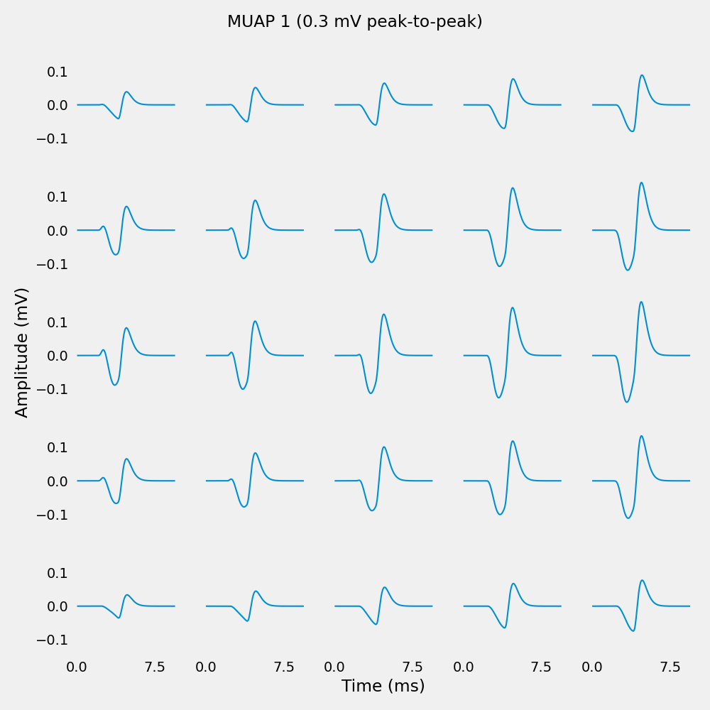
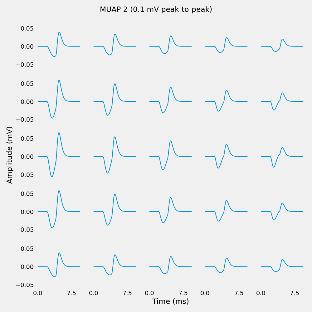
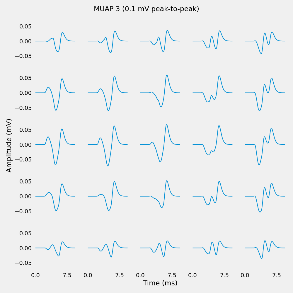
Plot MUAPs

Plot a single MUAP across the electrode grid. Each subplot shows the MUAP waveform at one electrode position.

# Select which MUAP to plot
for muap_index in range(len(muaps.groups[0].segments)):
    if np.mean(muaps.groups[0].segments[muap_index].analogsignals[0]) == 0:
        continue
    # Extract MUAP data from the Block object
    muap_signal = muaps.groups[0].segments[muap_index].analogsignals[0]
    muap_data_mV = muap_signal.magnitude  # Shape: (time, rows, cols)

    muap_data_uV = muap_signal.rescale(pq.uV).magnitude  # Convert to uV for plotting

    # Print amplitude diagnostics
    print(f"\nMUAP {muap_index} amplitude range:")
    print(f"\tMin: {np.min(muap_data_mV):.6f} mV ({np.min(muap_data_uV):.2f} uV)")
    print(f"\tMax: {np.max(muap_data_mV):.6f} mV ({np.max(muap_data_uV):.2f} uV)")
    print(f"\tPeak-to-peak: {np.ptp(muap_data_mV):.6f} mV ({np.ptp(muap_data_uV):.2f} uV)")

    # Get grid dimensions
    n_rows, n_cols = muap_data_uV.shape[1], muap_data_uV.shape[2]

    # Create subplot grid matching electrode layout
    fig, axs = plt.subplots(
        n_rows, n_cols, figsize=(n_cols * 2, n_rows * 2), sharex=True, sharey=True
    )
    fig.suptitle(f"MUAP {muap_index} ({np.ptp(muap_data_mV):.1f} mV peak-to-peak)")

    # get 100 ms around the center for better visualization (captures full MUAP waveform)
    time_vector = muap_signal.times.rescale(pq.ms).magnitude

    # Plot each electrode's waveform
    for row in range(n_rows):
        for col in range(n_cols):
            axs[row, col].plot(
                time_vector,
                muap_data_mV[:, row, col],
                linewidth=1.5,
            )
            axs[row, col].grid(False)
            if row == n_rows - 1 and col == n_cols // 2:
                axs[row, col].set_xticks([0, 7.5, 15])
                axs[row, col].set_xlabel("Time (ms)")
            if col == 0 and row == n_rows // 2:
                axs[row, col].set_ylabel("Amplitude (mV)")

    plt.tight_layout()
    plt.show()

• 
• 
• 
• 

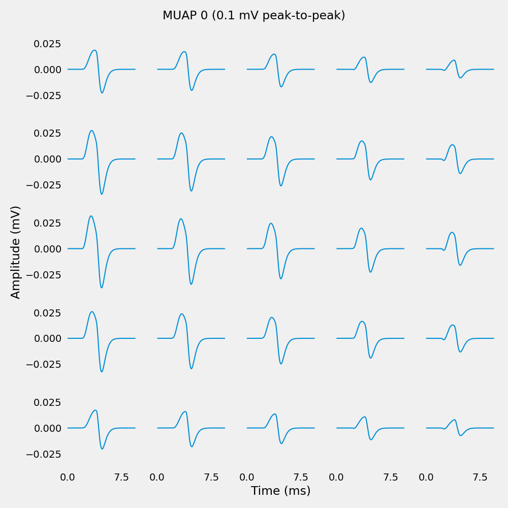
MUAP 0 amplitude range:
        Min: -0.037784 mV (-37.78 uV)
        Max: 0.031568 mV (31.57 uV)
        Peak-to-peak: 0.069352 mV (69.35 uV)

MUAP 1 amplitude range:
        Min: -0.139222 mV (-139.22 uV)
        Max: 0.160023 mV (160.02 uV)
        Peak-to-peak: 0.299245 mV (299.24 uV)

MUAP 2 amplitude range:
        Min: -0.056150 mV (-56.15 uV)
        Max: 0.066119 mV (66.12 uV)
        Peak-to-peak: 0.122270 mV (122.27 uV)

MUAP 3 amplitude range:
        Min: -0.072304 mV (-72.30 uV)
        Max: 0.067105 mV (67.10 uV)
        Peak-to-peak: 0.139409 mV (139.41 uV)