Current Generation

MyoGen provides various functions to generate different types of input currents for motor neuron pool simulations. These currents can be used to drive motor unit recruitment and firing patterns.

Note

Input currents are the electrical stimuli applied to motor neuron pools to simulate muscle activation. Different current shapes can produce different recruitment and firing patterns.

MyoGen offers 5 different current waveform types:

• Sinusoidal: Smooth oscillatory currents for rhythmic activation

• Sawtooth: Asymmetric ramp currents with adjustable rise/fall characteristics

• Step: Constant amplitude pulses for simple on/off activation

• Ramp: Linear increase/decrease for gradual force changes

• Trapezoid: Complex waveforms with rise, plateau, and fall phases

Import Libraries

from pathlib import Path

import joblib
import numpy as np
import quantities as pq
from matplotlib import pyplot as plt

from myogen.utils.currents import (
    create_ramp_current,
    create_sawtooth_current,
    create_sinusoidal_current,
    create_step_current,
    create_trapezoid_current,
)

plt.style.use("fivethirtyeight")

Define Parameters

Each current simulation is defined by common timing parameters:

• n_pools: Number of motor neuron pools

• simulation_duration__ms: Total simulation time in milliseconds

• timestep__ms: Time step for simulation in milliseconds

Additional parameters are specific to each current type and control amplitude, frequency, timing, and shape characteristics.

# Common simulation parameters
n_pools = 3
simulation_duration__ms = 2000.0  # 2 seconds
timestep__ms = 0.1  # 0.1 ms time step
t_points = int(simulation_duration__ms / timestep__ms)

# Create results directory
save_path = Path("./results")
save_path.mkdir(exist_ok=True)

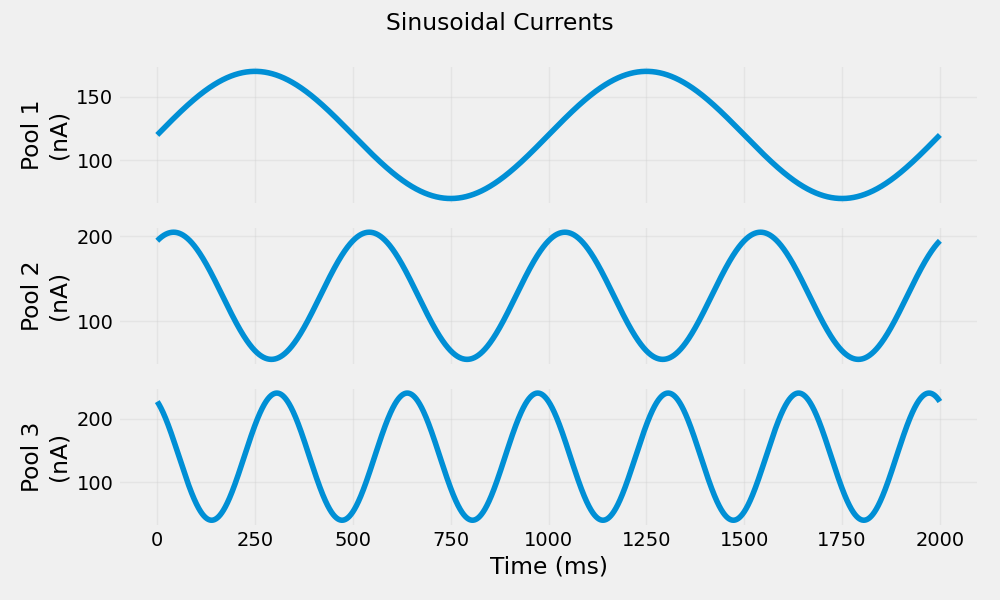
Generate Sinusoidal Currents

Sinusoidal currents are useful for simulating rhythmic muscle activations, such as those occurring during locomotion or tremor.

sinusoidal_currents = create_sinusoidal_current(
    n_pools=n_pools,
    t_points=t_points,
    timestep__ms=timestep__ms * pq.ms,
    amplitudes__nA=pq.Quantity([50.0, 75.0, 100.0], pq.nA),
    frequencies__Hz=pq.Quantity([1.0, 2.0, 3.0], pq.Hz),
    offsets__nA=pq.Quantity([120.0, 130.0, 140.0], pq.nA),
    phases__rad=pq.Quantity([0.0, np.pi / 3, 2 * np.pi / 3], pq.rad),
)

# Save to file
joblib.dump(sinusoidal_currents, save_path / "sinusoidal_currents.pkl")

# Plot sinusoidal currents
fig, axes = plt.subplots(n_pools, 1, figsize=(10, 6), sharex=True)
time_ms = sinusoidal_currents.times.rescale(pq.ms).magnitude
for i in range(n_pools):
    axes[i].plot(time_ms, sinusoidal_currents[:, i].magnitude)
    axes[i].set_ylabel(f"Pool {i + 1}\n(nA)")
    axes[i].grid(True, alpha=0.3)
axes[-1].set_xlabel("Time (ms)")
fig.suptitle("Sinusoidal Currents")
plt.tight_layout()
plt.show()

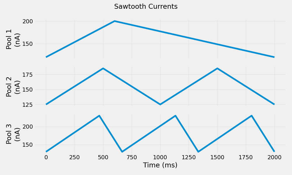
Generate Sawtooth Currents

Sawtooth currents provide asymmetric ramps useful for simulating force-variable contractions with different rise and fall characteristics.

sawtooth_currents = create_sawtooth_current(
    n_pools=n_pools,
    t_points=t_points,
    timestep__ms=timestep__ms * pq.ms,
    amplitudes__nA=pq.Quantity([80.0, 60.0, 100.0], pq.nA),
    frequencies__Hz=pq.Quantity([0.5, 1.0, 1.5], pq.Hz),
    offsets__nA=pq.Quantity([120.0, 125.0, 130.0], pq.nA),
    widths__ratio=[0.3, 0.5, 0.7],
)

# Save to file
joblib.dump(sawtooth_currents, save_path / "sawtooth_currents.pkl")

# Plot sawtooth currents
fig, axes = plt.subplots(n_pools, 1, figsize=(10, 6), sharex=True)
time_ms = sawtooth_currents.times.rescale(pq.ms).magnitude
for i in range(n_pools):
    axes[i].plot(time_ms, sawtooth_currents[:, i].magnitude)
    axes[i].set_ylabel(f"Pool {i + 1}\n(nA)")
    axes[i].grid(True, alpha=0.3)
axes[-1].set_xlabel("Time (ms)")
fig.suptitle("Sawtooth Currents")
plt.tight_layout()
plt.show()

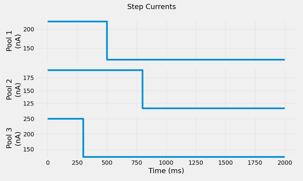
Generate Step Currents

Step currents are useful for simulating sudden muscle activations, such as those occurring during ballistic movements.

step_currents = create_step_current(
    n_pools=n_pools,
    t_points=t_points,
    timestep__ms=timestep__ms * pq.ms,
    step_heights__nA=pq.Quantity([100.0, 75.0, 125.0], pq.nA),
    step_durations__ms=pq.Quantity([500.0, 800.0, 300.0], pq.ms),
    offsets__nA=pq.Quantity([120.0, 115.0, 125.0], pq.nA),
)

# Save to file
joblib.dump(step_currents, save_path / "step_currents.pkl")

# Plot step currents
fig, axes = plt.subplots(n_pools, 1, figsize=(10, 6), sharex=True)
time_ms = step_currents.times.rescale(pq.ms).magnitude
for i in range(n_pools):
    axes[i].plot(time_ms, step_currents[:, i].magnitude)
    axes[i].set_ylabel(f"Pool {i + 1}\n(nA)")
    axes[i].grid(True, alpha=0.3)
axes[-1].set_xlabel("Time (ms)")
fig.suptitle("Step Currents")
plt.tight_layout()
plt.show()

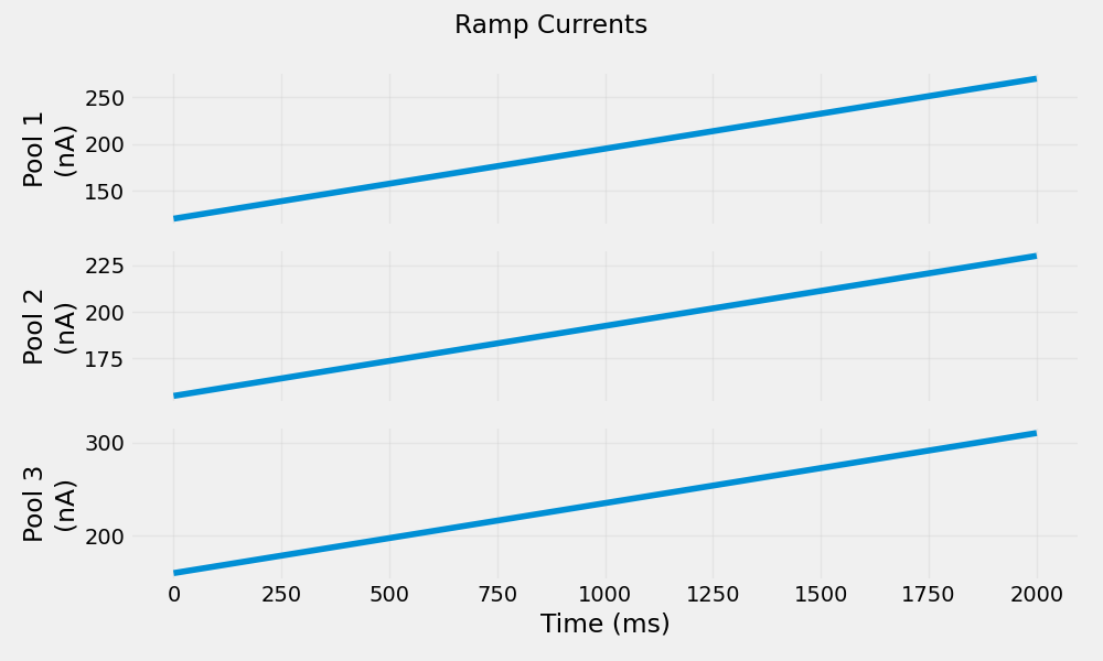
Generate Ramp Currents

Ramp currents simulate gradual force changes, useful for modeling slow force development or fatigue scenarios.

ramp_currents = create_ramp_current(
    n_pools=n_pools,
    t_points=t_points,
    timestep__ms=timestep__ms * pq.ms,
    start_currents__nA=pq.Quantity([0.0, 25.0, 50.0], pq.nA),
    end_currents__nA=pq.Quantity([150.0, 100.0, 200.0], pq.nA),
    offsets__nA=pq.Quantity([120.0, 130.0, 110.0], pq.nA),
)

# Save to file
joblib.dump(ramp_currents, save_path / "ramp_currents.pkl")

# Plot ramp currents
fig, axes = plt.subplots(n_pools, 1, figsize=(10, 6), sharex=True)
time_ms = ramp_currents.times.rescale(pq.ms).magnitude
for i in range(n_pools):
    axes[i].plot(time_ms, ramp_currents[:, i].magnitude)
    axes[i].set_ylabel(f"Pool {i + 1}\n(nA)")
    axes[i].grid(True, alpha=0.3)
axes[-1].set_xlabel("Time (ms)")
fig.suptitle("Ramp Currents")
plt.tight_layout()
plt.show()

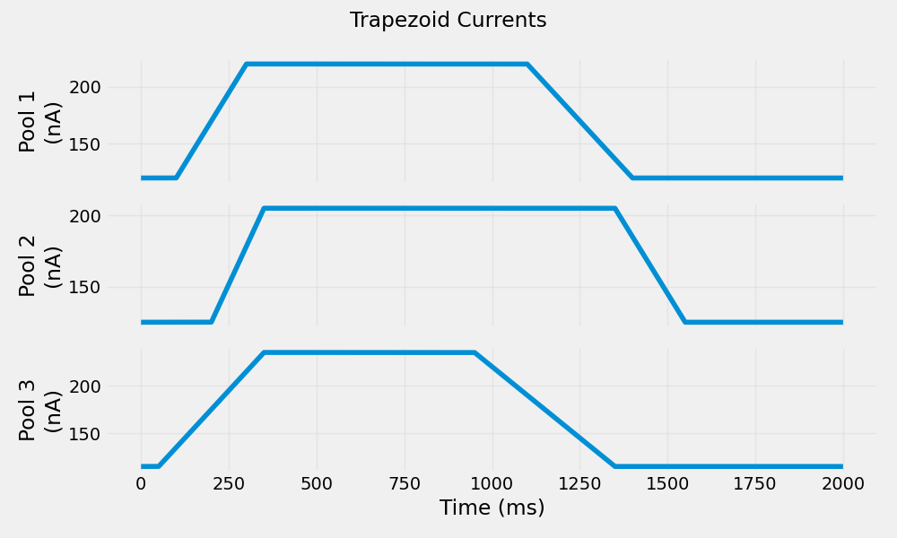
Generate Trapezoid Currents

Trapezoid currents provide complex activation patterns with distinct phases: rise, plateau, and fall. These are useful for simulating controlled muscle contractions.

trapezoid_currents = create_trapezoid_current(
    n_pools=n_pools,
    t_points=t_points,
    timestep__ms=timestep__ms * pq.ms,
    amplitudes__nA=pq.Quantity([100.0, 80.0, 120.0], pq.nA),
    rise_times__ms=pq.Quantity([200.0, 150.0, 300.0], pq.ms),
    plateau_times__ms=pq.Quantity([800.0, 1000.0, 600.0], pq.ms),
    fall_times__ms=pq.Quantity([300.0, 200.0, 400.0], pq.ms),
    offsets__nA=pq.Quantity([120.0, 125.0, 115.0], pq.nA),
    delays__ms=pq.Quantity([100.0, 200.0, 50.0], pq.ms),
)

# Save to file
joblib.dump(trapezoid_currents, save_path / "trapezoid_currents.pkl")

# Plot trapezoid currents
fig, axes = plt.subplots(n_pools, 1, figsize=(10, 6), sharex=True)
time_ms = trapezoid_currents.times.rescale(pq.ms).magnitude
for i in range(n_pools):
    axes[i].plot(time_ms, trapezoid_currents[:, i].magnitude)
    axes[i].set_ylabel(f"Pool {i + 1}\n(nA)")
    axes[i].grid(True, alpha=0.3)
axes[-1].set_xlabel("Time (ms)")
fig.suptitle("Trapezoid Currents")
plt.tight_layout()
plt.show()