Note
Click here to download the full example code
Loading and Inspecting NWB Data
This example demonstrates how to load, validate, and inspect NWB (Neurodata Without Borders) files created by MyoGen simulations.
NWB is a standardized data format for neurophysiology that enables: - Data sharing: Upload to DANDI Archive for community access - Interoperability: Compatible with many neuroscience analysis tools - Validation: Built-in schema validation ensures data integrity - Metadata: Rich experimental metadata travels with the data
Learning Objectives
- Validate NWB files: Use NWBInspector to check file compliance
- Load NWB data: Read simulation results back into Python
- Explore data structure: Navigate the hierarchical NWB format
- Extract signals: Access spike trains, analog signals, and metadata
- Compare formats: Understand NWB vs pickle tradeoffs
Prerequisites
This example requires an NWB file from example 11 (spinal_network_results.nwb).
Note
If you haven't run example 11, this example will create a minimal NWB file for demonstration purposes.
Import Libraries
from pathlib import Path

import matplotlib.pyplot as plt
import numpy as np

plt.style.use("fivethirtyeight")
Import NWB Libraries
import pynwb
from pynwb import NWBHDF5IO
from nwbinspector import inspect_nwbfile
from nwbinspector.inspector_tools import format_messages

print(f"(OK) PyNWB version: {pynwb.__version__}")
print("(OK) NWBInspector available")
Out:
/home/runner/work/MyoGen/MyoGen/examples/01_basic/13_load_and_inspect_nwb_data.py:53: DeprecationWarning: The 'inspector_tools' submodule has been deprecated. Please import the helper functions from the top-level package.
  from nwbinspector.inspector_tools import format_messages
(OK) PyNWB version: 3.1.3
(OK) NWBInspector available
Locate NWB File
Look for the NWB file created by example 11. If not found, we'll create a minimal example file for demonstration.
save_path = Path(r"./results")
nwb_filepath = save_path / "spinal_network_results.nwb"

if not nwb_filepath.exists():
    print(f"\n(WARN) NWB file not found: {nwb_filepath}")
    print("Creating a minimal demonstration NWB file...")

    # Create a minimal NWB file for demonstration
    from datetime import datetime, timezone

    import quantities as pq
    from neo import AnalogSignal, Block, Segment, SpikeTrain

    from myogen import get_random_generator
    from myogen.utils.nwb import export_to_nwb

    # Create sample data
    demo_block = Block(name="Demo_Simulation")
    segment = Segment(name="Demo_Segment")
    demo_block.segments.append(segment)

    # Add sample spike trains
    for i in range(5):
        spike_times = np.sort(get_random_generator().uniform(0, 1000, size=50)) * pq.ms
        st = SpikeTrain(spike_times, t_stop=1000 * pq.ms, units="ms")
        st.annotate(neuron_id=i, population="aMN")
        segment.spiketrains.append(st)

    # Add sample analog signal
    time_points = 10000
    signal_data = np.sin(np.linspace(0, 10 * np.pi, time_points)).reshape(-1, 1)
    analog = AnalogSignal(
        signal_data * pq.mV,
        sampling_rate=10000 * pq.Hz,
        name="muscle_force",
    )
    segment.analogsignals.append(analog)

    # Export to NWB
    save_path.mkdir(exist_ok=True)
    export_to_nwb(
        demo_block,
        nwb_filepath,
        session_description="Demonstration NWB file for MyoGen tutorial",
        institution="MyoGen Tutorial",
        # Pass an explicit session_start_time so the demo is fully reproducible
        # and avoids the new "no session_start_time" UserWarning.
        session_start_time=datetime(1970, 1, 1, tzinfo=timezone.utc),
    )
    print(f"(OK) Created demonstration NWB file: {nwb_filepath}")
else:
    print(f"\n(OK) Found NWB file: {nwb_filepath}")
    print(f"    Size: {nwb_filepath.stat().st_size / 1024:.1f} KB")
Out:
Step 1: Validate NWB File
Before loading, it's good practice to validate the NWB file using NWBInspector. This checks for schema compliance and best practices.
print("\n" + "=" * 60)
print("STEP 1: NWB FILE VALIDATION")
print("=" * 60)

print(f"\nValidating: {nwb_filepath.name}")
print("-" * 40)

# Run inspection
messages = list(inspect_nwbfile(nwbfile_path=str(nwb_filepath)))

if not messages:
    print("✓ No issues found - file is valid!")
else:
    # Categorize messages by severity
    critical = [m for m in messages if m.importance.name == "CRITICAL"]
    errors = [m for m in messages if m.importance.name == "ERROR"]
    warnings = [m for m in messages if m.importance.name == "WARNING"]
    best_practice = [m for m in messages if m.importance.name == "BEST_PRACTICE_VIOLATION"]

    print(f"Found {len(messages)} message(s):")
    if critical:
        print(f"  ✗ Critical: {len(critical)}")
    if errors:
        print(f"  ✗ Errors: {len(errors)}")
    if warnings:
        print(f"  ⚠ Warnings: {len(warnings)}")
    if best_practice:
        print(f"  ○ Best practice suggestions: {len(best_practice)}")

    # Show formatted messages
    print("\nDetails:")
    print(format_messages(messages[:10]))  # Limit to first 10
    if len(messages) > 10:
        print(f"  ... and {len(messages) - 10} more messages")
Out:
============================================================
STEP 1: NWB FILE VALIDATION
============================================================

Validating: spinal_network_results.nwb
----------------------------------------
Found 28 message(s):
  ✗ Critical: 3
  ○ Best practice suggestions: 1

Details:
['**************************************************', 'NWBInspector Report Summary', '', 'Timestamp: 2026-07-16 10:52:28.594440+00:00', 'Platform: Linux-6.17.0-1020-azure-x86_64-with-glibc2.39', 'NWBInspector version: 0.7.2', '', 'Found 10 issues across 1 file(s):', '       1 - BEST_PRACTICE_VIOLATION', '       9 - BEST_PRACTICE_SUGGESTION', '**************************************************', '', '', '0  results/spinal_network_results.nwb', '=====================================', '', "0.0  Importance.BEST_PRACTICE_VIOLATION: check_units_resolution_is_set - 'Units' object with name 'units'", '       Message: Units table has spike_times but resolution is not set. Resolution indicates the smallest possible difference between two spike times and should be a positive float equal to 1/sampling_rate of the recording system (e.g., Units(resolution=1/30000) for a 30 kHz system). This information is needed to assess the precision of spike timing data.', '', "0.1  Importance.BEST_PRACTICE_SUGGESTION: check_description - 'TimeSeries' object at location '/acquisition/spin_secondary_afferent_firing__Hz'", "       Message: Description ('no description') is a placeholder.", '', "0.2  Importance.BEST_PRACTICE_SUGGESTION: check_description - 'TimeSeries' object at location '/acquisition/spin_primary_afferent_firing__Hz'", "       Message: Description ('no description') is a placeholder.", '', "0.3  Importance.BEST_PRACTICE_SUGGESTION: check_description - 'TimeSeries' object at location '/acquisition/spin_intrafusal_tensions'", "       Message: Description ('no description') is a placeholder.", '', "0.4  Importance.BEST_PRACTICE_SUGGESTION: check_description - 'TimeSeries' object at location '/acquisition/spin_chain_activation'", "       Message: Description ('no description') is a placeholder.", '', "0.5  Importance.BEST_PRACTICE_SUGGESTION: check_description - 'TimeSeries' object at location '/acquisition/spin_bag2_activation'", "       Message: Description ('no description') is a placeholder.", '', "0.6  Importance.BEST_PRACTICE_SUGGESTION: check_description - 'TimeSeries' object at location '/acquisition/spin_bag1_activation'", "       Message: Description ('no description') is a placeholder.", '', "0.7  Importance.BEST_PRACTICE_SUGGESTION: check_description - 'TimeSeries' object at location '/acquisition/hill_muscle_type2_activation'", "       Message: Description ('no description') is a placeholder.", '', "0.8  Importance.BEST_PRACTICE_SUGGESTION: check_description - 'TimeSeries' object at location '/acquisition/hill_muscle_type1_activation'", "       Message: Description ('no description') is a placeholder.", '', "0.9  Importance.BEST_PRACTICE_SUGGESTION: check_description - 'TimeSeries' object at location '/acquisition/hill_muscle_muscle_torque'", "       Message: Description ('no description') is a placeholder.", '']
  ... and 18 more messages
Step 2: Load NWB File
Open the NWB file and explore its structure. NWB uses HDF5 format internally, which supports efficient storage of large datasets.
print("\n" + "=" * 60)
print("STEP 2: LOADING NWB FILE")
print("=" * 60)

# Open the NWB file
io = NWBHDF5IO(str(nwb_filepath), mode="r")
nwbfile = io.read()

print(f"\nNWB File: {nwbfile.identifier}")
print(f"Session: {nwbfile.session_description}")
print(f"Created: {nwbfile.session_start_time}")
if nwbfile.institution:
    print(f"Institution: {nwbfile.institution}")
if nwbfile.lab:
    print(f"Lab: {nwbfile.lab}")
if nwbfile.keywords:
    print(f"Keywords: {', '.join(nwbfile.keywords)}")
Out:
============================================================
STEP 2: LOADING NWB FILE
============================================================

NWB File: d99307bc-7a28-5b12-84b8-50abe1d59f93
Session: MyoGen spinal network simulation with systematic tendon tap protocol. Two-phase design: (1) Reflex gain modulation with varying gamma drive, (2) Reflex-voluntary interaction with sinusoidal cortical drive.
Created: 1970-01-01 00:00:00+00:00
Institution: MyoGen Framework
Lab: Neuromuscular Simulation
Keywords: MyoGen, spinal network, motor neuron, stretch reflex, tendon tap, proprioception, EMG simulation
Step 3: Explore Data Structure
NWB organizes data hierarchically. Let's explore what's available.
print("\n" + "=" * 60)
print("STEP 3: DATA STRUCTURE")
print("=" * 60)

# Acquisition data (raw recordings)
print("\n📁 Acquisition (raw data):")
if nwbfile.acquisition:
    for name, data in nwbfile.acquisition.items():
        print(f"  └─ {name}: {type(data).__name__}")
        if hasattr(data, "data"):
            print(f"      Shape: {data.data.shape if hasattr(data.data, 'shape') else 'N/A'}")
        if hasattr(data, "unit"):
            print(f"      Unit: {data.unit}")
else:
    print("  (empty)")

# Processing modules
print("\n📁 Processing modules:")
if nwbfile.processing:
    for mod_name, module in nwbfile.processing.items():
        print(f"  └─ {mod_name}:")
        for container_name in module.data_interfaces:
            container = module.data_interfaces[container_name]
            print(f"      └─ {container_name}: {type(container).__name__}")
else:
    print("  (empty)")

# Units (spike times)
print("\n📁 Units (spike data):")
if nwbfile.units is not None and len(nwbfile.units) > 0:
    n_units = len(nwbfile.units.id[:])
    print(f"  └─ {n_units} units recorded")
    # Show column names
    columns = list(nwbfile.units.colnames)
    print(f"      Columns: {', '.join(columns[:5])}")
    if len(columns) > 5:
        print(f"               ... and {len(columns) - 5} more")
else:
    print("  (empty)")

# Stimulus
print("\n📁 Stimulus:")
if nwbfile.stimulus:
    for name, data in nwbfile.stimulus.items():
        print(f"  └─ {name}: {type(data).__name__}")
else:
    print("  (empty)")
Out:
============================================================
STEP 3: DATA STRUCTURE
============================================================

📁 Acquisition (raw data):
  └─ aMN_cell0_Vm: TimeSeries
      Shape: (1000001, 1)
      Unit: mV
  └─ aMN_cell10_Vm: TimeSeries
      Shape: (1000001, 1)
      Unit: mV
  └─ aMN_cell15_Vm: TimeSeries
      Shape: (1000001, 1)
      Unit: mV
  └─ aMN_cell20_Vm: TimeSeries
      Shape: (1000001, 1)
      Unit: mV
  └─ aMN_cell30_Vm: TimeSeries
      Shape: (1000001, 1)
      Unit: mV
  └─ aMN_cell40_Vm: TimeSeries
      Shape: (1000001, 1)
      Unit: mV
  └─ aMN_cell50_Vm: TimeSeries
      Shape: (1000001, 1)
      Unit: mV
  └─ aMN_cell5_Vm: TimeSeries
      Shape: (1000001, 1)
      Unit: mV
  └─ aMN_cell60_Vm: TimeSeries
      Shape: (1000001, 1)
      Unit: mV
  └─ aMN_cell70_Vm: TimeSeries
      Shape: (1000001, 1)
      Unit: mV
  └─ gto_ib_afferent_firing__Hz: TimeSeries
      Shape: (1000001, 1)
      Unit: dimensionless
  └─ hill_muscle_muscle_force: TimeSeries
      Shape: (1000001, 1)
      Unit: dimensionless
  └─ hill_muscle_muscle_length: TimeSeries
      Shape: (1000001, 1)
      Unit: dimensionless
  └─ hill_muscle_muscle_torque: TimeSeries
      Shape: (1000001, 1)
      Unit: dimensionless
  └─ hill_muscle_type1_activation: TimeSeries
      Shape: (1000001, 1)
      Unit: dimensionless
  └─ hill_muscle_type2_activation: TimeSeries
      Shape: (1000001, 1)
      Unit: dimensionless
  └─ spin_bag1_activation: TimeSeries
      Shape: (1000001, 1)
      Unit: dimensionless
  └─ spin_bag2_activation: TimeSeries
      Shape: (1000001, 1)
      Unit: dimensionless
  └─ spin_chain_activation: TimeSeries
      Shape: (1000001, 1)
      Unit: dimensionless
  └─ spin_intrafusal_tensions: TimeSeries
      Shape: (3, 1000001)
      Unit: dimensionless
  └─ spin_primary_afferent_firing__Hz: TimeSeries
      Shape: (1000001, 1)
      Unit: dimensionless
  └─ spin_secondary_afferent_firing__Hz: TimeSeries
      Shape: (1000001, 1)
      Unit: dimensionless

📁 Processing modules:
  (empty)

📁 Units (spike data):
  └─ 966 units recorded
      Columns: _name, segment, block, spike_times, obs_intervals

📁 Stimulus:
  (empty)
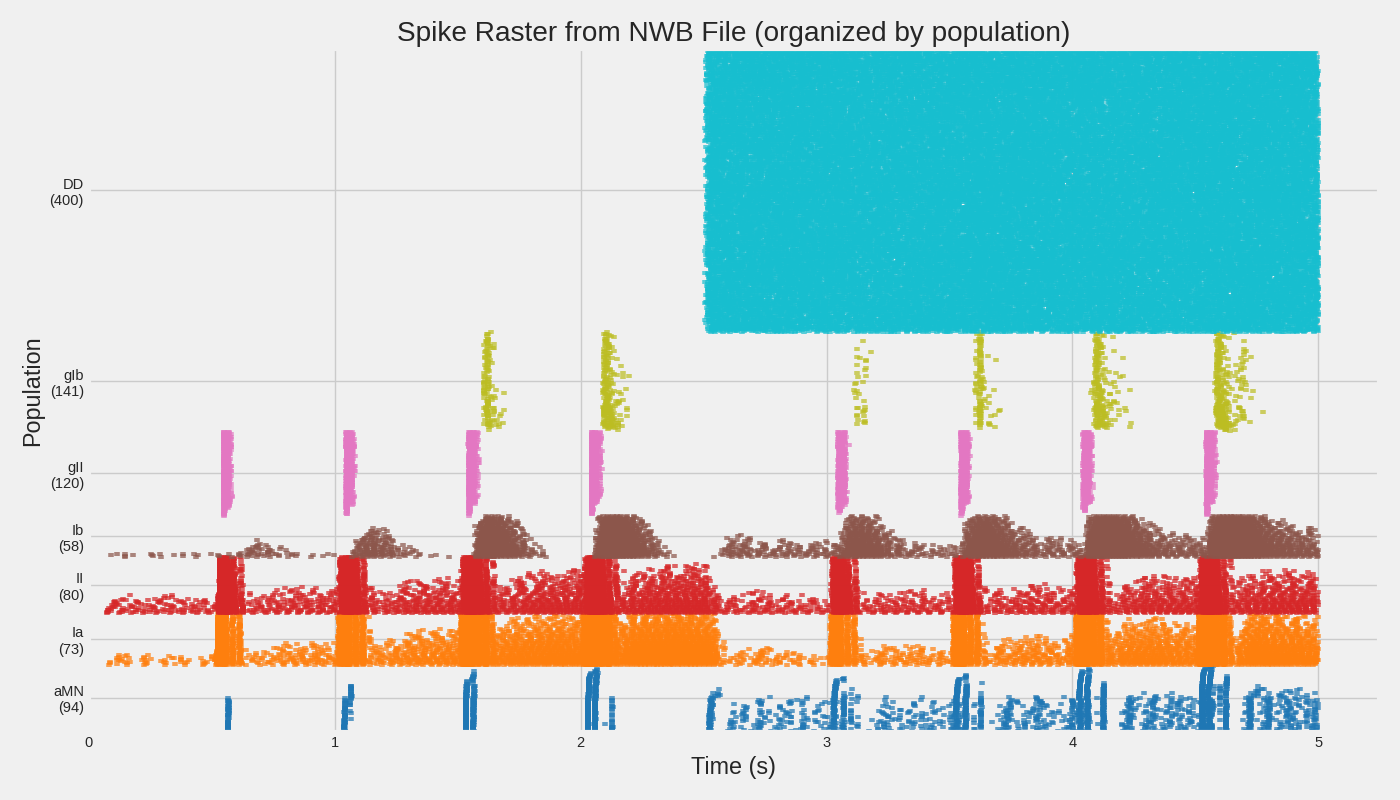
Step 4: Extract and Plot Spike Data
If the NWB file contains spike data, let's extract and visualize it.
print("\n" + "=" * 60)
print("STEP 4: EXTRACTING SPIKE DATA")
print("=" * 60)

if nwbfile.units is not None and len(nwbfile.units) > 0:
    # Get unit info - names contain population info like "aMN_cell0_spikes"
    unit_ids = nwbfile.units.id[:]
    unit_names = nwbfile.units["_name"][:] if "_name" in nwbfile.units.colnames else None

    print(f"\nFound {len(unit_ids)} units")

    # Group units by population (parse from name like "aMN_cell0_spikes")
    populations = {}
    for i, unit_id in enumerate(unit_ids):
        name = unit_names[i] if unit_names is not None else f"unit_{unit_id}"
        # Parse population from "popName_cellN_spikes" format
        if "_cell" in name:
            pop_name = name.split("_cell")[0]
        else:
            pop_name = "unknown"

        if pop_name not in populations:
            populations[pop_name] = []

        spike_times = nwbfile.units.get_unit_spike_times(unit_id)
        populations[pop_name].append((name, spike_times))

    print(f"Populations found: {list(populations.keys())}")
    for pop, units in populations.items():
        total_spikes = sum(len(st) for _, st in units)
        print(f"  {pop}: {len(units)} units, {total_spikes} total spikes")

    # Create raster plot organized by population (like example 11)
    pop_order = ["aMN", "Ia", "II", "Ib", "gII", "gIb"]  # Preferred order
    sorted_pops = [p for p in pop_order if p in populations]
    sorted_pops += [p for p in populations if p not in sorted_pops]  # Add any others

    fig, ax = plt.subplots(figsize=(14, 8))
    colors = plt.cm.tab10(np.linspace(0, 1, len(sorted_pops)))

    y_offset = 0
    y_ticks = []
    y_labels = []

    for pop_idx, pop_name in enumerate(sorted_pops):
        units = populations[pop_name]
        pop_start_y = y_offset

        for unit_name, spike_times in units:
            if len(spike_times) > 0:
                ax.scatter(
                    spike_times,
                    np.ones_like(spike_times) * y_offset,
                    marker="|",
                    s=8,
                    color=colors[pop_idx],
                    alpha=0.7,
                )
            y_offset += 1

        # Add population label at midpoint
        y_ticks.append((pop_start_y + y_offset) / 2)
        y_labels.append(f"{pop_name}\n({len(units)})")

    ax.set_xlabel("Time (s)")
    ax.set_ylabel("Population")
    ax.set_yticks(y_ticks)
    ax.set_yticklabels(y_labels)
    ax.set_title("Spike Raster from NWB File (organized by population)")
    ax.set_xlim(0, None)
    ax.set_ylim(-1, y_offset)

    plt.tight_layout()
    plt.savefig(save_path / "nwb_spike_raster.png", dpi=150, bbox_inches="tight")
    plt.show()
    print(f"\n(OK) Saved raster plot to: {save_path / 'nwb_spike_raster.png'}")
else:
    print("\nNo spike data found in this NWB file")
Out:
============================================================
STEP 4: EXTRACTING SPIKE DATA
============================================================

Found 966 units
Populations found: ['DD', 'aMN', 'Ia', 'II', 'Ib', 'gII', 'gIb']
  DD: 400 units, 40000 total spikes
  aMN: 94 units, 2087 total spikes
  Ia: 73 units, 11846 total spikes
  II: 80 units, 8685 total spikes
  Ib: 58 units, 4651 total spikes
  gII: 120 units, 1930 total spikes
  gIb: 141 units, 889 total spikes

(OK) Saved raster plot to: results/nwb_spike_raster.png
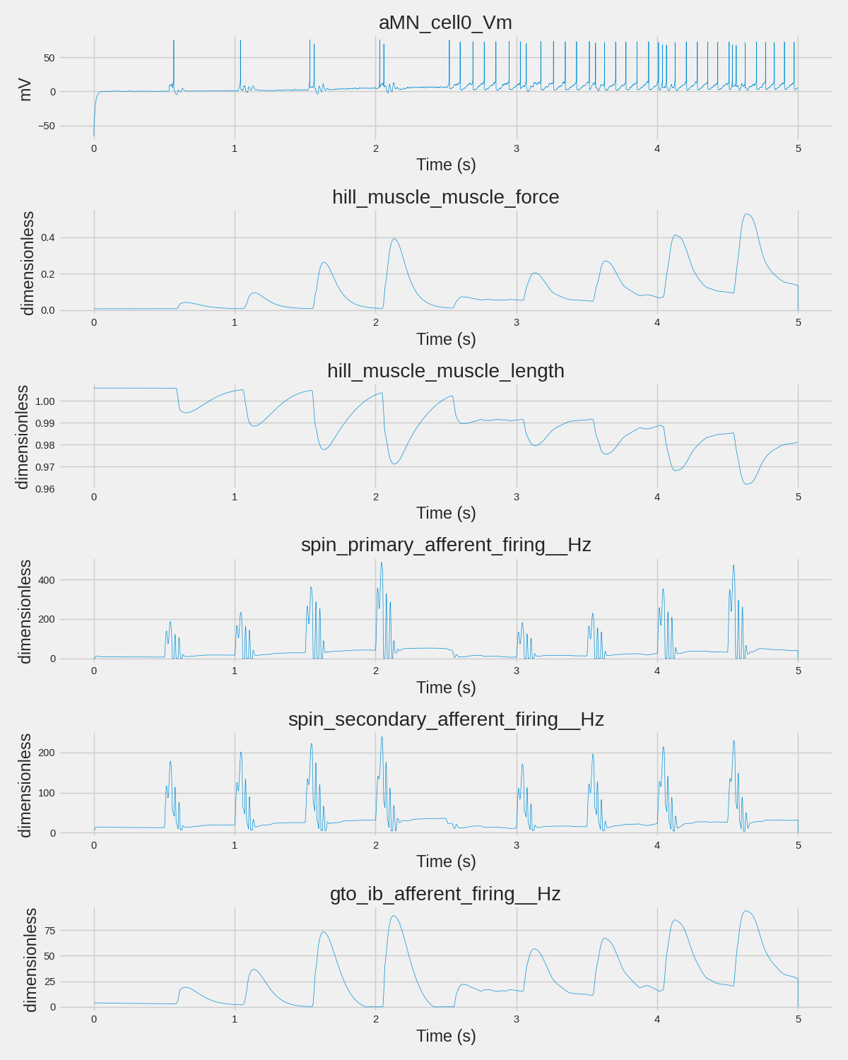
Step 5: Extract and Plot Analog Signals
Let's look at any continuous time series data in the file.
print("\n" + "=" * 60)
print("STEP 5: EXTRACTING ANALOG SIGNALS")
print("=" * 60)


def get_timestamps(data):
    """Get timestamps from NWB TimeSeries, handling both explicit and rate-based."""
    if data.timestamps is not None:
        return data.timestamps[:]
    elif data.rate is not None:
        # Generate timestamps from starting_time and rate
        n_samples = data.data.shape[0]
        start = data.starting_time if data.starting_time is not None else 0.0
        return np.linspace(start, start + n_samples / data.rate, n_samples)
    else:
        # Fallback to sample indices
        return np.arange(data.data.shape[0])


# Check acquisition for time series
analog_signals = []
for name, data in nwbfile.acquisition.items():
    if hasattr(data, "data"):
        analog_signals.append((name, data))

print(f"\nFound {len(analog_signals)} analog signals in acquisition:")
for name, data in analog_signals[:10]:  # Show first 10
    print(f"  - {name}: shape={data.data.shape}, unit={getattr(data, 'unit', 'N/A')}")
if len(analog_signals) > 10:
    print(f"  ... and {len(analog_signals) - 10} more")

# Select representative signals from different categories
signals_to_plot = []
signal_dict = {name: data for name, data in analog_signals}

# Pick one from each category for a representative view
representative_patterns = [
    "aMN_cell0_Vm",  # Membrane potential
    "hill_muscle_muscle_force",  # Muscle force
    "hill_muscle_muscle_length",  # Muscle length
    "spin_primary_afferent_firing__Hz",  # Spindle Ia
    "spin_secondary_afferent_firing__Hz",  # Spindle II
    "gto_ib_afferent_firing__Hz",  # GTO Ib
]

for pattern in representative_patterns:
    if pattern in signal_dict:
        signals_to_plot.append((pattern, signal_dict[pattern]))

# Fallback to first 4 if no matches
if not signals_to_plot:
    signals_to_plot = analog_signals[:4]

if signals_to_plot:
    print(f"\nPlotting {len(signals_to_plot)} representative signals...")
    fig, axes = plt.subplots(len(signals_to_plot), 1, figsize=(12, 2.5 * len(signals_to_plot)))
    if len(signals_to_plot) == 1:
        axes = [axes]

    for ax, (name, data) in zip(axes, signals_to_plot):
        values = data.data[:]
        if values.ndim > 1:
            values = values[:, 0]  # Take first channel if multi-channel
        timestamps = get_timestamps(data)

        ax.plot(timestamps, values, linewidth=0.5)
        ax.set_xlabel("Time (s)")
        ax.set_ylabel(f"{getattr(data, 'unit', 'a.u.')}")
        ax.set_title(name)

    plt.tight_layout()
    plt.savefig(save_path / "nwb_analog_signals.png", dpi=150, bbox_inches="tight")
    plt.show()
    print(f"(OK) Saved analog signal plot to: {save_path / 'nwb_analog_signals.png'}")
else:
    print("\nNo analog signals found in acquisition")
Out:
============================================================
STEP 5: EXTRACTING ANALOG SIGNALS
============================================================

Found 22 analog signals in acquisition:
  - aMN_cell0_Vm: shape=(1000001, 1), unit=mV
  - aMN_cell10_Vm: shape=(1000001, 1), unit=mV
  - aMN_cell15_Vm: shape=(1000001, 1), unit=mV
  - aMN_cell20_Vm: shape=(1000001, 1), unit=mV
  - aMN_cell30_Vm: shape=(1000001, 1), unit=mV
  - aMN_cell40_Vm: shape=(1000001, 1), unit=mV
  - aMN_cell50_Vm: shape=(1000001, 1), unit=mV
  - aMN_cell5_Vm: shape=(1000001, 1), unit=mV
  - aMN_cell60_Vm: shape=(1000001, 1), unit=mV
  - aMN_cell70_Vm: shape=(1000001, 1), unit=mV
  ... and 12 more

Plotting 6 representative signals...
(OK) Saved analog signal plot to: results/nwb_analog_signals.png
Step 6: Compare with Pickle Format
Let's compare loading from NWB vs the original pickle format.
print("\n" + "=" * 60)
print("STEP 6: NWB vs PICKLE COMPARISON")
print("=" * 60)

pickle_filepath = save_path / "spinal_network_results.pkl"

print("\nFormat Comparison:")
print("-" * 50)
print(f"{'Feature':<25} {'NWB':<15} {'Pickle':<15}")
print("-" * 50)

# File existence
nwb_exists = "✓" if nwb_filepath.exists() else "✗"
pkl_exists = "✓" if pickle_filepath.exists() else "✗"
print(f"{'File exists':<25} {nwb_exists:<15} {pkl_exists:<15}")

# File size
if nwb_filepath.exists():
    nwb_size = f"{nwb_filepath.stat().st_size / 1024:.1f} KB"
else:
    nwb_size = "N/A"
if pickle_filepath.exists():
    pkl_size = f"{pickle_filepath.stat().st_size / 1024:.1f} KB"
else:
    pkl_size = "N/A"
print(f"{'File size':<25} {nwb_size:<15} {pkl_size:<15}")

# Format properties
print(f"{'Standardized format':<25} {'Yes':<15} {'No':<15}")
print(f"{'Schema validation':<25} {'Yes':<15} {'No':<15}")
print(f"{'Cross-language support':<25} {'Yes (HDF5)':<15} {'Python only':<15}")
print(f"{'DANDI Archive upload':<25} {'Yes':<15} {'No':<15}")
print(f"{'Metadata schema':<25} {'Rich':<15} {'Flexible':<15}")
print(f"{'Load speed':<25} {'Fast':<15} {'Fast':<15}")
print("-" * 50)

print("\nRecommendations:")
print("  • Use NWB for: Sharing data, long-term archival, interoperability")
print("  • Use Pickle for: Quick local saves, complex Python objects, development")
Out:
============================================================
STEP 6: NWB vs PICKLE COMPARISON
============================================================

Format Comparison:
--------------------------------------------------
Feature                   NWB             Pickle
--------------------------------------------------
File exists               ✓               ✓
File size                 188458.0 KB     188361.8 KB
Standardized format       Yes             No
Schema validation         Yes             No
Cross-language support    Yes (HDF5)      Python only
DANDI Archive upload      Yes             No
Metadata schema           Rich            Flexible
Load speed                Fast            Fast
--------------------------------------------------

Recommendations:
  • Use NWB for: Sharing data, long-term archival, interoperability
  • Use Pickle for: Quick local saves, complex Python objects, development
Cleanup
Close the NWB file handle.
Out:
Summary
This example demonstrated:
- Validation: Using NWBInspector to check file compliance
- Loading: Opening NWB files with PyNWB
- Structure exploration: Navigating the hierarchical format
- Data extraction: Accessing spikes and analog signals
- Format comparison: Understanding NWB vs pickle tradeoffs
For more information:
- NWB documentation: https://pynwb.readthedocs.io/
- NWBInspector: https://nwbinspector.readthedocs.io/
- DANDI Archive: https://dandiarchive.org/
- NWB Overview: https://nwb-overview.readthedocs.io/
print("\n" + "=" * 60)
print("EXAMPLE COMPLETE")
print("=" * 60)
print("\nNext steps:")
print("  1. Run example 11 to generate full simulation NWB file")
print("  2. Explore your data with NWB Widgets: pip install nwbwidgets")
print("  3. Upload to DANDI Archive for sharing: https://dandiarchive.org/")
Out:
============================================================
EXAMPLE COMPLETE
============================================================

Next steps:
  1. Run example 11 to generate full simulation NWB file
  2. Explore your data with NWB Widgets: pip install nwbwidgets
  3. Upload to DANDI Archive for sharing: https://dandiarchive.org/
Total running time of the script: ( 0 minutes 5.539 seconds)
Download Python source code: 13_load_and_inspect_nwb_data.py