Note

Click here to download the full example code

Spike Train Generation with Descending Drive

This example simulates motor neuron spike trains driven by a descending drive (DD): a population of Poisson neurons modelling cortical input, connected to the motor neuron pool through synapses. This is more realistic than direct current injection (example 02) because it models the synaptic input from upper motor neurons.

The drive here is the calibrated FDI drive of the fdi_semg profile card: its network, noise and drive rates were fitted so the pool recruits and fires like a human first dorsal interosseous, and the card maps force levels in % MVC to drive. One call runs it.

Note

The card is myogen/profiles/fdi_semg.yaml: every value with its source, and notes on what else to check when you change one. load_profile("fdi_semg.published") gives each component as its source paper describes it. To build the pools yourself, see card.motor_neuron_pool() and myogen.simulator.neuron.descending_drive_network.

Import Libraries

Important

In MyoGen all random number generation is handled by the RNG returned from get_random_generator, a thin wrapper around numpy.random. The profile card reseeds it from its own seeds before each build, so a card run is reproducible.

from pathlib import Path

import joblib
import numpy as np
import quantities as pq
from matplotlib import pyplot as plt
from neo import AnalogSignal

from myogen import load_profile
from myogen.utils.nmodl import load_nmodl_mechanisms

plt.style.use("fivethirtyeight")


def mean_firing_rate(spiketrain):
    """Mean firing rate of a neo.SpikeTrain (replaces elephant.statistics.mean_firing_rate)."""
    return (len(spiketrain) / (spiketrain.t_stop - spiketrain.t_start)).rescale(pq.Hz)


def population_psth(spiketrains, bin_size):
    """Total spike counts per bin across spiketrains, plus bin left edges (s).

    Native replacement for elephant.statistics.time_histogram (output="counts").
    """
    t_start = min(st.t_start for st in spiketrains).rescale(pq.s).magnitude
    t_stop = max(st.t_stop for st in spiketrains).rescale(pq.s).magnitude
    bs = (bin_size).rescale(pq.s).magnitude
    n_bins = int((t_stop - t_start) / bs)
    edges = t_start + np.arange(n_bins + 1) * bs
    spikes = np.concatenate([st.rescale(pq.s).magnitude for st in spiketrains])
    spikes = spikes[(spikes >= edges[0]) & (spikes < edges[-1])]  # drop right-edge spikes
    counts, _ = np.histogram(spikes, bins=edges)
    return counts, edges[:-1]

Run the Calibrated Drive

A trapezoidal contraction to 25 % MVC: 1 s rest, 4 s ramp up, 4 s hold, 4 s ramp down, 1 s rest. Each segment is (duration_s, start_pct_mvc, end_pct_mvc).

Note

This runs 120 biophysical motor neurons for 14 s and takes a few minutes.

load_nmodl_mechanisms()

save_path = Path("./results")
save_path.mkdir(exist_ok=True)

card = load_profile()  # fdi_semg
protocol = [(1, 0, 0), (4, 0, 25), (4, 25, 25), (4, 25, 0), (1, 0, 0)]
result = card.simulate(protocol)

spike_train_block = result.spikes
mn_segment = spike_train_block.segments[0]
n_motor_neurons = len(mn_segment.spiketrains)
simulation_time = sum(d for d, _, _ in protocol) * pq.s
timestep = float(card.value("drive.timestep_ms")) * pq.ms
ramp_up_end = 5.0 * pq.s  # start of the hold
plateau_end = 9.0 * pq.s  # end of the hold

# Excitation (0-1) per drive time step, saved for the surface EMG example
excitation_signal = AnalogSignal(result.excitation[:, None], units=pq.dimensionless,
                                 sampling_period=timestep.rescale(pq.s))

# The spike trains and the excitation are used by the surface EMG example (06) and the force example (08)
joblib.dump(spike_train_block, save_path / "trapezoid_dd_spike_trains.pkl")
joblib.dump(excitation_signal, save_path / "trapezoid_drive_pattern.pkl")

Out:

['results/trapezoid_drive_pattern.pkl']

Calculate Firing Rate Statistics

mn_firing_rates = np.array(
    [
        mean_firing_rate(st__s.time_slice(st__s.min(), st__s.max()))
        for st__s in mn_segment.spiketrains
        if len(st__s) > 1  # need >=2 spikes for a rate over the spike span
    ]
)

print("Motor neurons:")
print(f"\tActive neurons: {len(mn_firing_rates)}/{n_motor_neurons}")
if len(mn_firing_rates) > 0:
    print(f"\tMean firing rate: {np.mean(mn_firing_rates):.1f} ± {np.std(mn_firing_rates):.1f} pps")
    print(f"\tRate range: {np.min(mn_firing_rates):.1f} - {np.max(mn_firing_rates):.1f} pps")

Out:

Motor neurons:
        Active neurons: 103/120
        Mean firing rate: 13.3 ± 2.9 pps
        Rate range: 1.9 - 15.6 pps

Visualization

1. Target force and the simulated force (% MVC)
2. Motor neuron raster plot showing recruitment
3. Population firing rate over time

fig, axes = plt.subplots(3, 1, figsize=(15, 10), sharex=True)

t_force = np.arange(result.force_pct_mvc.size) / result.fs_force__Hz
t_target = np.cumsum([0] + [d for d, _, _ in protocol])
target = [protocol[0][1]] + [b for _, _, b in protocol]
axes[0].plot(t_target, target, "k--", linewidth=2, label="Target")
axes[0].plot(t_force, result.force_pct_mvc, "b-", linewidth=2, label="Force")
axes[0].set_ylabel("Force (% MVC)")
axes[0].set_title("Trapezoidal Contraction (calibrated FDI drive)")
axes[0].legend()
axes[0].grid(True, alpha=0.3)

mn_colors = plt.get_cmap("Reds")(np.linspace(0.3, 0.9, n_motor_neurons))
active_mn_count = 0
for i, (spiketrain, color) in enumerate(zip(mn_segment.spiketrains, mn_colors)):
    if len(spiketrain) > 0:
        spike_times = spiketrain.rescale(pq.s).magnitude
        axes[1].scatter(spike_times, [i] * len(spike_times), c=[color], s=1.0, alpha=0.8)
        active_mn_count += 1

axes[1].set_ylabel("Motor Neuron ID\n(Recruitment Order)")
axes[1].set_title(f"Motor Neuron Population Activity (n={active_mn_count}/{n_motor_neurons} active)")
axes[1].set_ylim(-1, n_motor_neurons)
axes[1].grid(True, alpha=0.3)

bin_size_ms = 100
mn_counts, bin_centers_s = population_psth(mn_segment.spiketrains, bin_size_ms * pq.ms)
mn_rates_binned = mn_counts / (bin_size_ms / 1000.0) / n_motor_neurons
axes[2].plot(bin_centers_s, mn_rates_binned, "r-", linewidth=2, label="MN Population", alpha=0.8)
axes[2].set_xlabel("Time (s)")
axes[2].set_ylabel("Population Rate (Hz)")
axes[2].set_title("Population Firing Rate Over Time")
axes[2].legend()
axes[2].grid(True, alpha=0.3)

for ax in axes:
    ax.set_xlim(0, simulation_time.rescale(pq.s).magnitude)

plt.tight_layout()
plt.show()

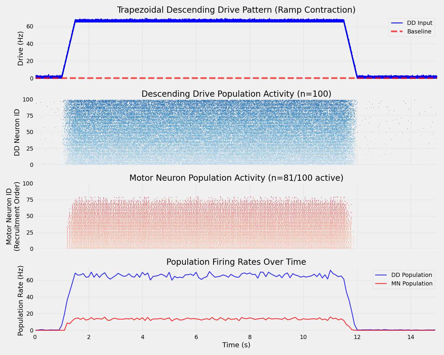
Individual Motor Neuron Discharge Rates

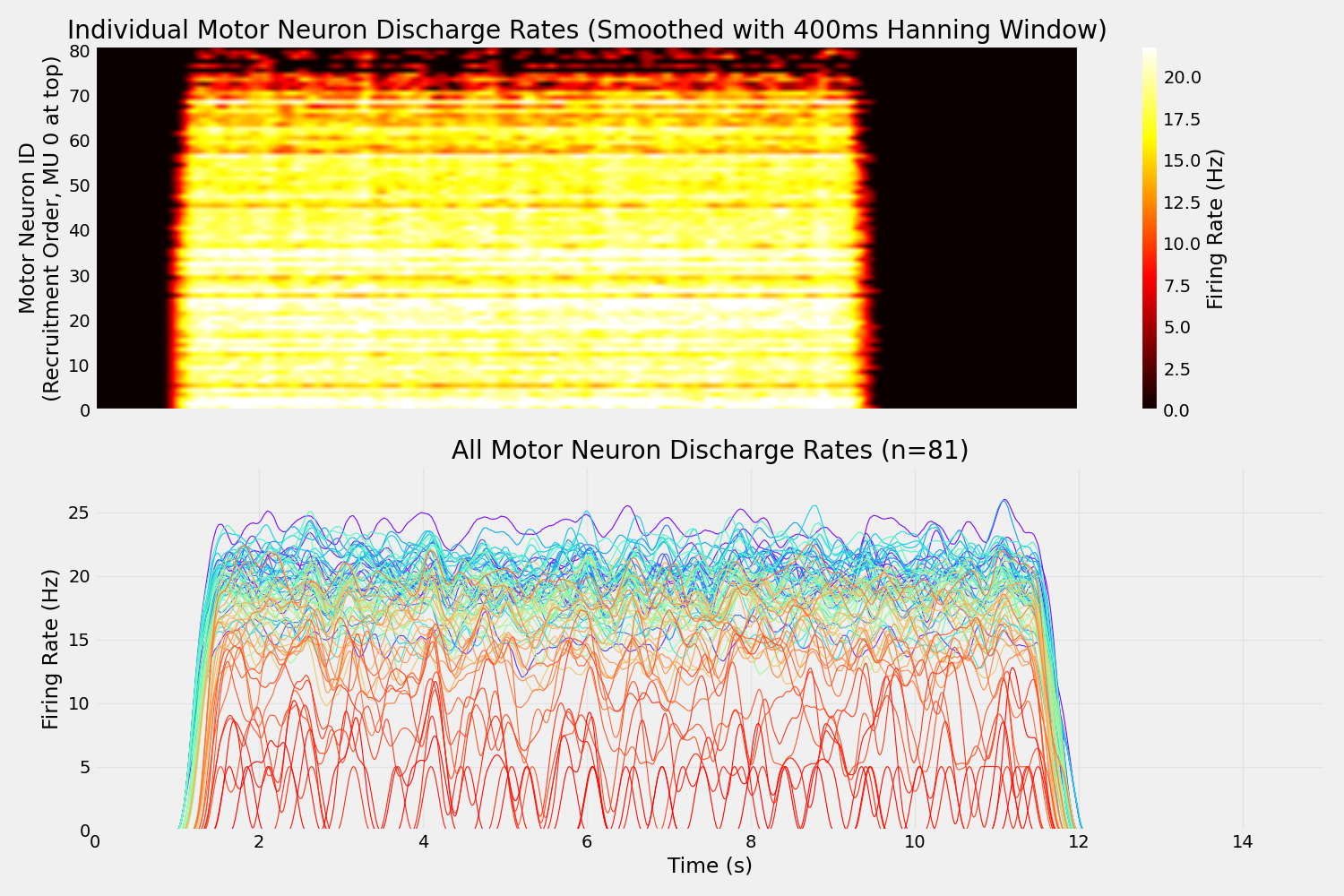
Compute smoothed instantaneous firing rates for each motor neuron with a 400 ms Hanning window.

print("\nComputing smoothed discharge rates per neuron...")

# Parameters
window_ms = 400 * pq.ms  # 400 ms Hanning window
dt_s = timestep.rescale(pq.s)  # simulation timestep in seconds
window_samples = int(window_ms.rescale(pq.s) / dt_s)

# Hanning window normalized to preserve rate
hanning_window = np.hanning(window_samples)
hanning_window = hanning_window / (hanning_window.sum() * dt_s)  # convert to Hz

mn_instantaneous_rates = []
active_neuron_ids = []

mean_firing_rates = []
cv_isi = []

for i, spiketrain in enumerate(mn_segment.spiketrains):
    if len(spiketrain) > 2:
        # Convert spike times to a binary spike train
        t = np.arange(0, simulation_time.rescale(pq.s).magnitude, dt_s.magnitude)
        spikes = np.zeros_like(t)
        spike_indices = np.searchsorted(t, spiketrain.magnitude)
        spikes[spike_indices[spike_indices < len(t)]] = 1

        # Convolve with Hanning window
        rate = np.convolve(spikes, hanning_window, mode="same")
        mn_instantaneous_rates.append(rate)
        active_neuron_ids.append(i)

        # IMPORTANT: Compute ISI/CV only during plateau phase where firing is stable
        # Filter spike train to plateau phase
        plateau_spiketrain = spiketrain.time_slice(ramp_up_end, plateau_end)

        # Compute mean firing rate (Hz) from plateau spikes only
        plateau_duration_s = float((plateau_end - ramp_up_end).rescale(pq.s).magnitude)
        mean_rate = (
            len(plateau_spiketrain) / plateau_duration_s if len(plateau_spiketrain) > 0 else 0.0
        )
        mean_firing_rates.append(mean_rate)

        # Compute CV of inter-spike intervals (plateau phase only)
        if len(plateau_spiketrain) > 1:
            spike_times = plateau_spiketrain.rescale(pq.s).magnitude
            isis = np.diff(spike_times)
            cv = np.std(isis) / np.mean(isis) if len(isis) > 1 else 0.0
        else:
            cv = 0.0
        cv_isi.append(cv)

# Population averages
pop_mean_rate = np.mean(mean_firing_rates)
pop_mean_cv = np.mean(cv_isi)
print(f"\nPopulation: Mean firing rate = {pop_mean_rate:.2f} Hz, CV = {pop_mean_cv:.2f}")

print(f"  Computed rates for {len(active_neuron_ids)} active motor neurons")

# Create new figure for individual discharge rates
fig2, axes2 = plt.subplots(2, 1, figsize=(15, 10), sharex=True)

# 1. Heatmap of instantaneous firing rates
if len(mn_instantaneous_rates) > 0:
    # Stack rates into 2D array (neurons x time)
    rates_array = np.array(mn_instantaneous_rates)
    time_points = np.linspace(0, simulation_time.rescale(pq.s).magnitude, rates_array.shape[1])

    # Plot heatmap (with origin='lower' so MU 0 is at TOP)
    im = axes2[0].imshow(
        rates_array,
        aspect="auto",
        cmap="hot",
        interpolation="bilinear",
        extent=[0, simulation_time.rescale(pq.s).magnitude, 0, len(active_neuron_ids)],
        origin="lower",  # Puts first row (MU 0) at bottom, but we'll flip with extent
        vmin=0,
        vmax=np.percentile(rates_array, 95),
    )

    axes2[0].set_ylabel("Motor Neuron ID\n(Recruitment Order, MU 0 at top)")
    axes2[0].set_title(
        "Individual Motor Neuron Discharge Rates (Smoothed with 400ms Hanning Window)"
    )
    # Add colorbar
    cbar = plt.colorbar(im, ax=axes2[0])
    cbar.set_label("Firing Rate (Hz)")
    axes2[0].grid(False)

    # 2. Individual traces
    n_to_plot = len(active_neuron_ids)

    # Use colormap for lines (gradient from blue to red showing recruitment order)
    colors = plt.get_cmap("rainbow")(np.linspace(0, 1, n_to_plot))

    for neuron_idx in range(n_to_plot):
        axes2[1].plot(
            time_points,
            mn_instantaneous_rates[neuron_idx],
            linewidth=0.8,
            color=colors[neuron_idx],
            label=f"MN {active_neuron_ids[neuron_idx]}" if n_to_plot <= 20 else None,
        )

    axes2[1].set_xlabel("Time (s)")
    axes2[1].set_ylabel("Firing Rate (Hz)")
    axes2[1].set_title(f"All Motor Neuron Discharge Rates (n={n_to_plot})")

    # Only show legend if there are few neurons
    if n_to_plot <= 20:
        axes2[1].legend(loc="upper right", ncol=3, fontsize=6)

    axes2[1].grid(True, alpha=0.3)
    axes2[1].set_xlim(0, simulation_time.rescale(pq.s).magnitude)
    axes2[1].set_ylim(0, np.max(rates_array) * 1.1)

plt.tight_layout()
plt.show()

print("\n[DONE] Simulation complete with discharge rate analysis!")

Out:

Computing smoothed discharge rates per neuron...

Population: Mean firing rate = 16.57 Hz, CV = 0.25
  Computed rates for 103 active motor neurons

[DONE] Simulation complete with discharge rate analysis!

Total running time of the script: ( 0 minutes 29.583 seconds)

Download Python source code: 03_simulate_spike_trains_descending_drive.py

Gallery generated by mkdocs-gallery