Force Generation

After generating spike trains from motor neuron pools, the next step is to simulate the force output produced by the muscle. MyoGen provides a comprehensive force model based on the classic Fuglevand et al. (1993) approach.

Note

The force model converts spike trains into force by simulating individual motor unit twitches and their summation. Each motor unit has unique twitch characteristics (amplitude, duration) that depend on its recruitment threshold.

The force model includes:

• Motor unit twitch characteristics: Peak force and contraction time based on recruitment thresholds

• Nonlinear gain modulation: Force scaling based on inter-pulse intervals (discharge rate)

• Temporal summation: Realistic force buildup from overlapping twitches

• Physiological scaling: Realistic force ranges and dynamics

References

[1]

Fuglevand, A. J., Winter, D. A., & Patla, A. E. (1993). Models of recruitment and rate coding in motor-unit pools. Journal of Neurophysiology, 70(2), 782-797.

Import Libraries

from pathlib import Path

import numpy as np
import matplotlib.pyplot as plt

from myogen import simulator
from myogen.simulator.core.force.force_model import ForceModel
from myogen.utils.plotting.force import (
    plot_twitch_parameter_assignment,
    plot_twitches,
)
from myogen.utils.plotting import plot_spike_trains
from myogen.utils.currents import create_trapezoid_current

Define Parameters

The force model requires several key parameters:

• recruitment_thresholds: Motor unit recruitment thresholds

• recording_frequency__Hz: Sampling frequency for force simulation

• longest_duration_rise_time__ms: Maximum twitch rise time

• contraction_time_range: Range of contraction times across motor units

For demonstration, we’ll also create input currents and simulate the complete pipeline from current input to force output.

# Create results directory
save_path = Path("./results")
save_path.mkdir(exist_ok=True)

# Motor unit pool parameters
n_motor_units = 100
recruitment_range = 100  # Recruitment range (max_threshold / min_threshold)

# Force model parameters
recording_frequency__Hz = 10000.0  # 10 kHz sampling rate
longest_duration_rise_time__ms = 90.0  # Maximum twitch rise time
contraction_time_range = 3.0  # Contraction time range factor

# Simulation parameters
simulation_duration__ms = 10000.0  # 10 seconds
timestep__ms = 0.1  # 0.1 ms time step
t_points = int(simulation_duration__ms / timestep__ms)

Generate Recruitment Thresholds

First, we need to generate recruitment thresholds for our motor unit pool. These will determine both the activation order and the force characteristics of each motor unit.

recruitment_thresholds, _ = simulator.generate_mu_recruitment_thresholds(
    N=n_motor_units, recruitment_range__ratio=recruitment_range
)

Create Force Model

The force model calculates individual motor unit twitch properties based on recruitment thresholds and physiological scaling rules.

force_model = ForceModel(
    recruitment_thresholds=recruitment_thresholds,
    recording_frequency__Hz=recording_frequency__Hz,
    longest_duration_rise_time__ms=longest_duration_rise_time__ms,
    contraction_time_range__unitless=contraction_time_range,
)

# Display force model statistics
print(f"\nForce model statistics:")
print(f"  - Number of motor units: {force_model._number_of_neurons}")
print(f"  - Recruitment ratio: {force_model._recruitment_ratio:.1f}")
print(
    f"  - Peak force range: {force_model.peak_twitch_forces__unitless[0]:.3f} - {force_model.peak_twitch_forces__unitless[-1]:.3f}"
)
print(
    f"  - Contraction time range: {force_model.contraction_times__samples[0]:.1f} - {force_model.contraction_times__samples[-1]:.1f} samples"
)

Force model statistics:
  - Number of motor units: 100
  - Recruitment ratio: 100.0
  - Peak force range: 1.047 - 100.000
  - Contraction time range: 890.2 - 300.0 samples

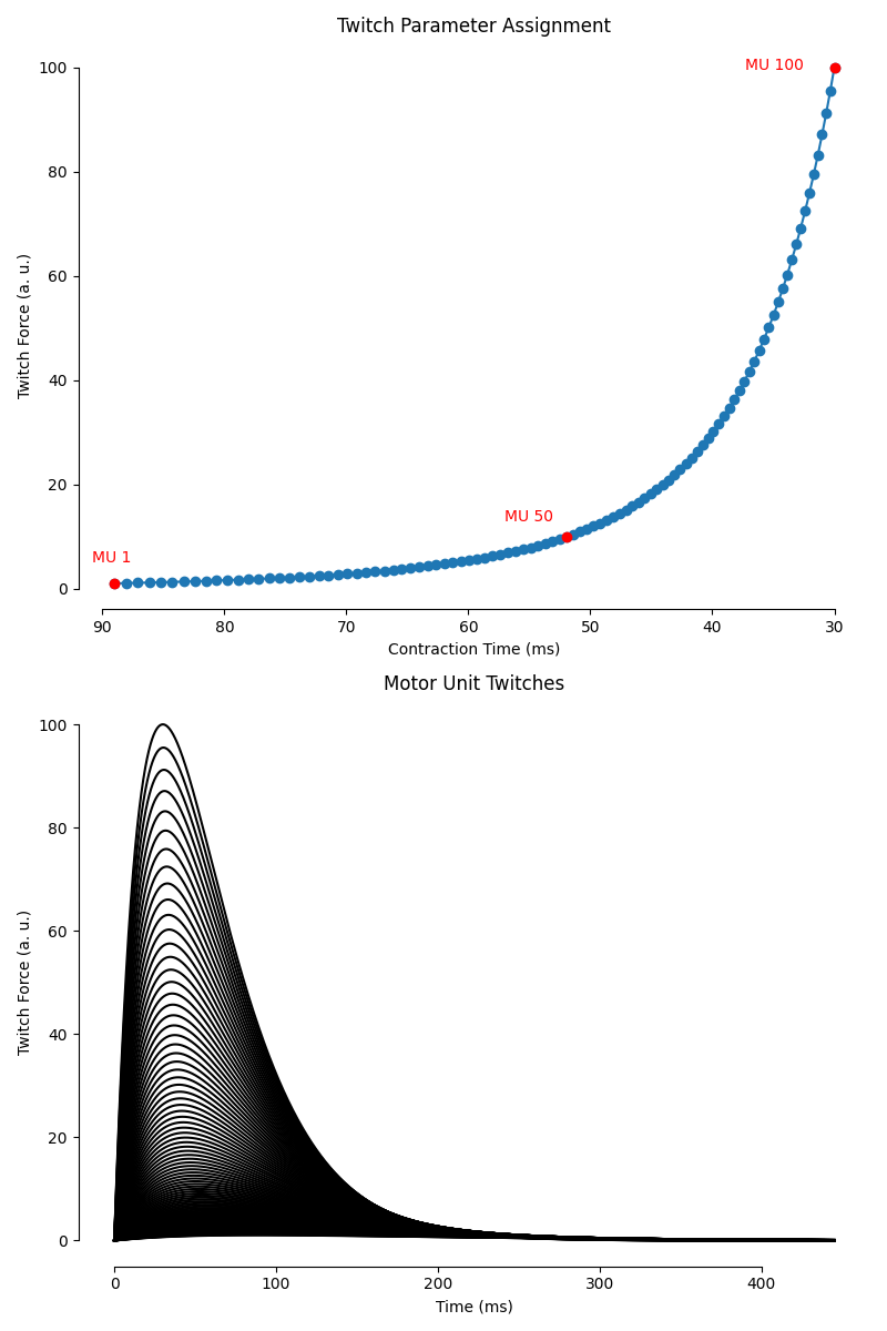
Visualize Twitch Parameter Assignment

The force model assigns twitch parameters (peak force and contraction time) to each motor unit based on its recruitment threshold. Let’s visualize this relationship for a subset of motor units.

# Suppress font warnings to keep output clean
import warnings
import logging

warnings.filterwarnings("ignore", message=".*Font family.*not found.*")
warnings.filterwarnings("ignore", message=".*findfont.*")
logging.getLogger("matplotlib.font_manager").setLevel(logging.ERROR)

plt.figure(figsize=(8, 12))

ax1 = plt.subplot(2, 1, 1)
plot_twitch_parameter_assignment(
    force_model, ax1, [1, 50, 100], flip_x=True, apply_default_formatting=True
)
ax1.set_title("Twitch Parameter Assignment")

ax2 = plt.subplot(2, 1, 2)
plot_twitches(force_model, ax2, apply_default_formatting=True)
ax2.set_title("Motor Unit Twitches")

plt.tight_layout()
plt.show()

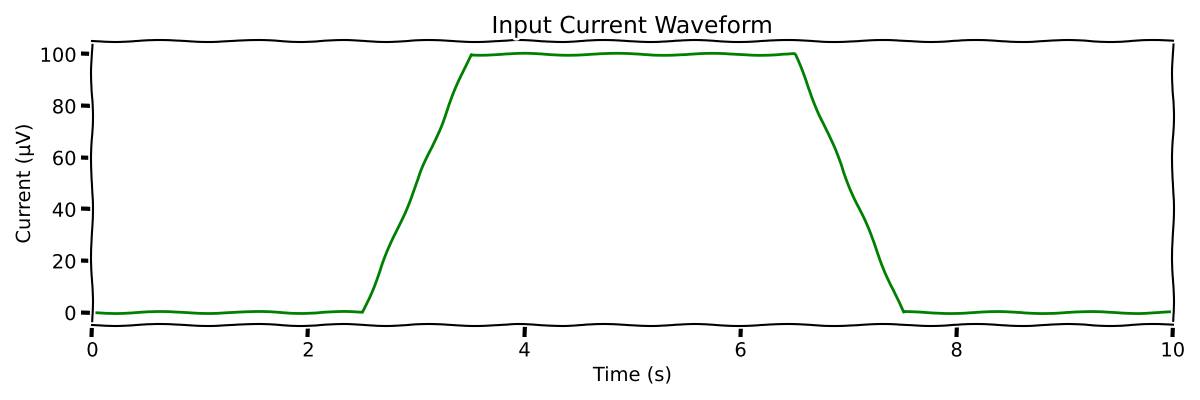
Generate Input Current

To demonstrate force generation, we’ll create a trapezoid current that will drive motor unit recruitment and firing patterns.

# Parameters for trapezoid current
trap_amplitude = 100.0  # Peak amplitude
trap_rise_time = 1000.0  # Rise duration (ms)
trap_plateau_time = 3000.0  # Plateau duration (ms)
trap_fall_time = 1000.0  # Fall duration (ms)
trap_offset = 0.0  # Baseline current
trap_delay = 2500.0  # Initial delay (ms)

trapezoid_current = create_trapezoid_current(
    n_pools=1,
    t_points=t_points,
    timestep__ms=timestep__ms,
    amplitudes__muV=[trap_amplitude],
    rise_times__ms=[trap_rise_time],
    plateau_times__ms=[trap_plateau_time],
    fall_times__ms=[trap_fall_time],
    offsets__muV=[trap_offset],
    delays__ms=[trap_delay],
)

# Plot the input current
plt.figure(figsize=(12, 4))
with plt.xkcd():
    time_vector = np.arange(t_points) * timestep__ms / 1000  # Convert to seconds
    plt.plot(time_vector, trapezoid_current[0], "g-", linewidth=2)
    plt.xlabel("Time (s)")
    plt.ylabel("Current (µV)")
    plt.title("Input Current Waveform")
    plt.grid(True, alpha=0.3)
    plt.xlim(0, simulation_duration__ms / 1000)

plt.tight_layout()
plt.show()

Create Motor Neuron Pool and Generate Spike Trains

Now we’ll create a motor neuron pool and generate spike trains in response to the input current.

# Create motor neuron pool
motor_neuron_pool = simulator.MotorNeuronPool(recruitment_thresholds)

# Generate spike trains
spike_trains_matrix, active_neuron_indices, data = (
    motor_neuron_pool.generate_spike_trains(
        input_current__matrix=trapezoid_current,
        timestep__ms=timestep__ms,
        noise_mean__nA=0.0,
        noise_stdev__nA=0.0,
    )
)

Creating motor neuron pools:   0%|          | 0/1 [00:00<?, ?pool/s]
Creating motor neuron pools: 100%|██████████| 1/1 [00:00<00:00, 24.62pool/s]

Injecting currents into pools:   0%|          | 0/1 [00:00<?, ?pool/s]

Adding noise to neurons in pool:   0%|          | 0/100 [00:00<?, ?neuron/s]

Adding noise to neurons in pool:  21%|██        | 21/100 [00:00<00:00, 204.81neuron/s]

Adding noise to neurons in pool:  42%|████▏     | 42/100 [00:00<00:00, 203.57neuron/s]

Adding noise to neurons in pool:  63%|██████▎   | 63/100 [00:00<00:00, 204.59neuron/s]

Adding noise to neurons in pool:  84%|████████▍ | 84/100 [00:00<00:00, 205.31neuron/s]


Injecting currents into pools: 100%|██████████| 1/1 [00:00<00:00,  1.63pool/s]
Injecting currents into pools: 100%|██████████| 1/1 [00:00<00:00,  1.63pool/s]

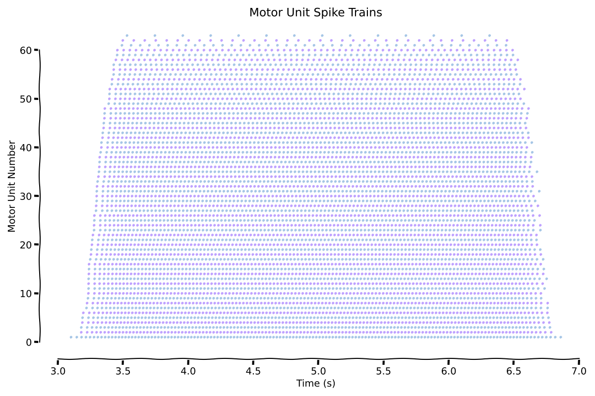
Visualize Spike Trains

Let’s visualize the generated spike trains to see the motor unit recruitment and firing patterns.

plt.figure(figsize=(12, 8))

with plt.xkcd():
    ax = plt.gca()
    plot_spike_trains(spike_trains_matrix, timestep__ms, [ax])
    ax.set_title("Motor Unit Spike Trains")
    ax.set_xlabel("Time (s)")
    ax.set_ylabel("Motor Unit Number")

plt.tight_layout()
plt.show()

Generate Force Output

Now we can use the force model to convert the spike trains into force output. The model will simulate individual motor unit twitches and their temporal summation to produce the total muscle force.

# Generate force from spike trains
force_output = force_model.generate_force(spike_trains_matrix)

# Add some realistic noise to the force signal
noise_level = 0.015  # 0.5% of mean force
noisy_force = force_output[0] + np.random.randn(
    len(force_output[0])
) * noise_level * np.mean(force_output[0])

Twitch trains are generated:   0%|          | 0/100 [00:00<?, ?it/s]
Twitch trains are generated:   9%|▉         | 9/100 [00:00<00:01, 85.19it/s]
Twitch trains are generated:  18%|█▊        | 18/100 [00:00<00:00, 85.47it/s]
Twitch trains are generated:  27%|██▋       | 27/100 [00:00<00:00, 85.71it/s]
Twitch trains are generated:  36%|███▌      | 36/100 [00:00<00:00, 86.43it/s]
Twitch trains are generated:  45%|████▌     | 45/100 [00:00<00:00, 87.06it/s]
Twitch trains are generated:  55%|█████▌    | 55/100 [00:00<00:00, 88.14it/s]
Twitch trains are generated:  65%|██████▌   | 65/100 [00:00<00:00, 89.25it/s]
Twitch trains are generated:  75%|███████▌  | 75/100 [00:00<00:00, 91.45it/s]
Twitch trains are generated:  85%|████████▌ | 85/100 [00:00<00:00, 92.30it/s]
Twitch trains are generated:  95%|█████████▌| 95/100 [00:01<00:00, 92.45it/s]
Twitch trains are generated: 100%|██████████| 100/100 [00:01<00:00, 89.92it/s]

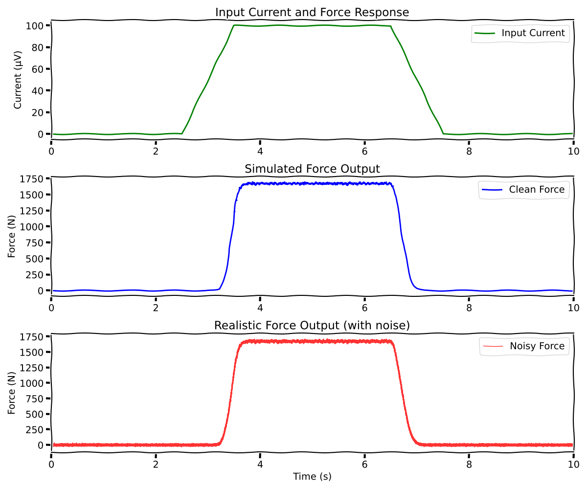
Visualize Force Output

Let’s plot the generated force alongside the input current to see how the muscle responds to the electrical stimulation.

plt.figure(figsize=(12, 10))

with plt.xkcd():
    # Plot input current
    ax1 = plt.subplot(3, 1, 1)
    ax1.plot(
        time_vector, trapezoid_current[0], "g-", linewidth=2, label="Input Current"
    )
    ax1.set_ylabel("Current (µV)")
    ax1.set_title("Input Current and Force Response")
    ax1.grid(True, alpha=0.3)
    ax1.legend()
    ax1.set_xlim(0, simulation_duration__ms / 1000)

    # Plot clean force
    ax2 = plt.subplot(3, 1, 2)
    ax2.plot(time_vector, force_output[0], "b-", linewidth=2, label="Clean Force")
    ax2.set_ylabel("Force (N)")
    ax2.set_title("Simulated Force Output")
    ax2.grid(True, alpha=0.3)
    ax2.legend()
    ax2.set_xlim(0, simulation_duration__ms / 1000)

    # Plot noisy force (more realistic)
    ax3 = plt.subplot(3, 1, 3)
    ax3.plot(
        time_vector, noisy_force, "r-", linewidth=1, alpha=0.8, label="Noisy Force"
    )
    ax3.set_xlabel("Time (s)")
    ax3.set_ylabel("Force (N)")
    ax3.set_title("Realistic Force Output (with noise)")
    ax3.grid(True, alpha=0.3)
    ax3.legend()
    ax3.set_xlim(0, simulation_duration__ms / 1000)

plt.tight_layout()
plt.show()