Complex filtering

This example shows how to apply a complex filter sequence to the data.

Loading data and selection one task for simplicity

Just as in the previous example we load the EMG example data and convert it to a MyoVerse Data object. Afterward, we select one task to work with.

import pickle as pkl
from copy import copy

import numpy as np

from myoverse.datatypes import EMGData

emg_data = {}
with open("data/emg.pkl", "rb") as f:
    for k, v in pkl.load(f).items():
        emg_data[k] = EMGData(v, sampling_frequency=2044)

print(emg_data)

task_one_data = copy(emg_data["1"])

print(task_one_data)

{'1': EMGData; Sampling frequency: 2044 Hz; (0) Input (320, 20440), '2': EMGData; Sampling frequency: 2044 Hz; (0) Input (320, 20440)}
--
EMGData
Sampling frequency: 2044 Hz
(0) Input (320, 20440)
--

Applying a basic filter sequence

A common filter sequence used by us in our deep learning papers is to first apply a bandpass between 47.5 and 52.5 Hz to remove the powerline noise.

Then we copied this filtered data and applied a lowpass filter at 20 Hz to remove high-frequency noise. The deep learning models were thus trained with 2 representations of the data, one with the powerline noise removed and one with the high-frequency noise removed.

We can achieve this by applying two filters to the data using the apply_filters method.

Note

Please run this code on your local machine as the plots are interactive and information can be seen by hovering over the nodes.

from scipy.signal import butter

from myoverse.datasets.filters.temporal import SOSFrequencyFilter

# Define the filters
bandpass_filter = SOSFrequencyFilter(
    sos_filter_coefficients=butter(4, [47.5, 52.5], "bandpass", output="sos", fs=2044),
    is_output=True,
    name="Bandpass 50",
)
lowpass_filter = SOSFrequencyFilter(
    sos_filter_coefficients=butter(4, 20, "lowpass", output="sos", fs=2044),
    is_output=True,
    name="Lowpass 20",
)

# Apply the filters
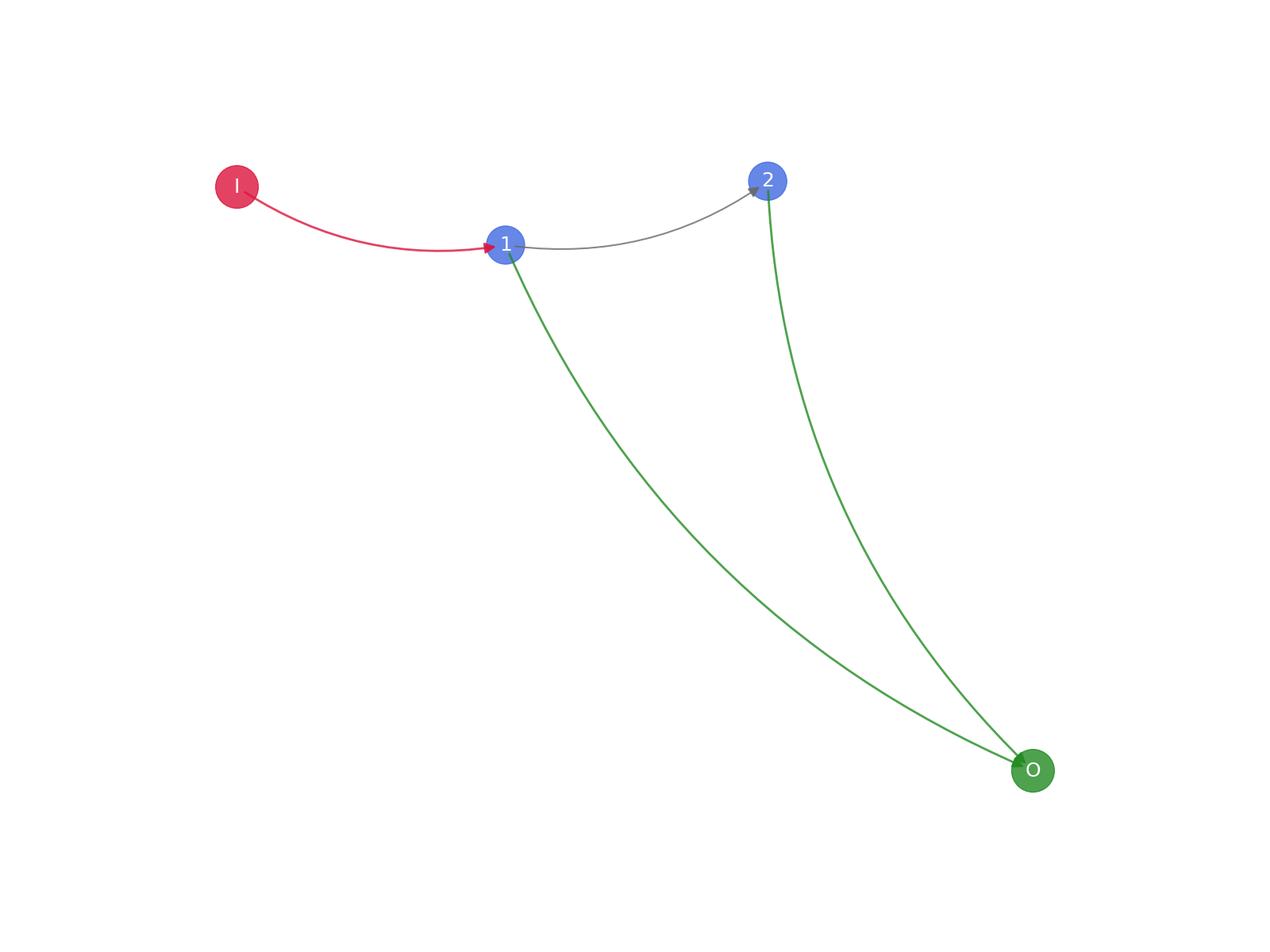
task_one_data.apply_filter_sequence(
    filter_sequence=[bandpass_filter, lowpass_filter], representation_to_filter="Input"
)

print()
print(task_one_data)

task_one_data.plot_graph()

--
EMGData
Sampling frequency: 2044 Hz
(0) Input (320, 20440)

Filter(s):
(1 | 1) (Output) Bandpass 50 (320, 20440)
(2 | 1 -> 2) (Output) Lowpass 20 (320, 20440)
--

Applying a complex filter sequence

In this example we will apply a more complex filter sequence to the data.

The filter shall apply the following steps:

1. Chunk the data into 100 ms windows.

2. Apply a bandpass filter between 47.5 and 52.5 Hz to remove powerline noise.

3. Copy the filtered data and apply a lowpass filter at 20 Hz to remove high-frequency noise.

4. Compute the root mean square of the data from step 3.

5. The other copy of step 2 should be used to calculate the root mean square directly.

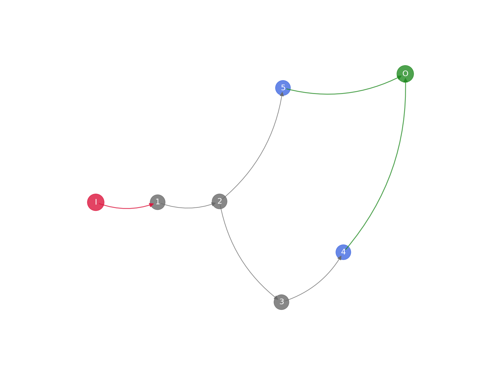
The computation graph for this filter sequence is shown below:

1 -> 2 -> 3 -> 4

L ——–> 5

We can achieve this by applying five filters to the data using the apply_filter_sequence method and setting the is_output flag to True for the filters that should be kept in the dataset object.

from myoverse.datasets.filters.generic import ChunkizeDataFilter, ApplyFunctionFilter
from myoverse.datasets.filters.temporal import SOSFrequencyFilter

# reset the data
task_one_data = copy(emg_data["1"])

# Define the filters
bandpass_filter = butter(4, [47.5, 52.5], "bandpass", output="sos", fs=2044)
lowpass_filter = butter(4, 20, "lowpass", output="sos", fs=2044)

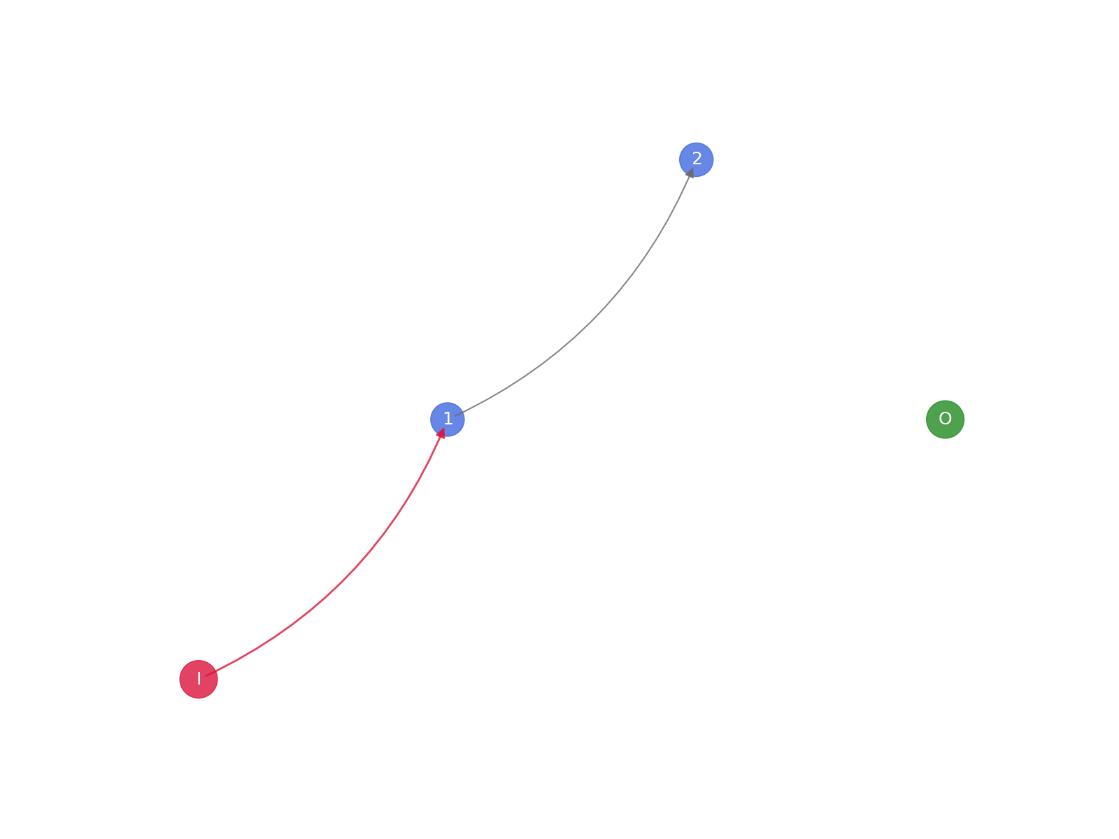
Apply the filters for steps 1 and 2

task_one_data.apply_filter_sequence(
    filter_sequence=[
        ChunkizeDataFilter(chunk_size=192, chunk_shift=64),
        SOSFrequencyFilter(sos_filter_coefficients=bandpass_filter, name="Bandpass 50"),
    ],
    representation_to_filter="Input",
)

print(task_one_data)

task_one_data.plot_graph()

--
EMGData
Sampling frequency: 2044 Hz
(0) Input (320, 20440)

Filter(s):
(1 | 1) ChunkizeDataFilter (317, 320, 192)
(2 | 1 -> 2) Bandpass 50 (317, 320, 192)
--

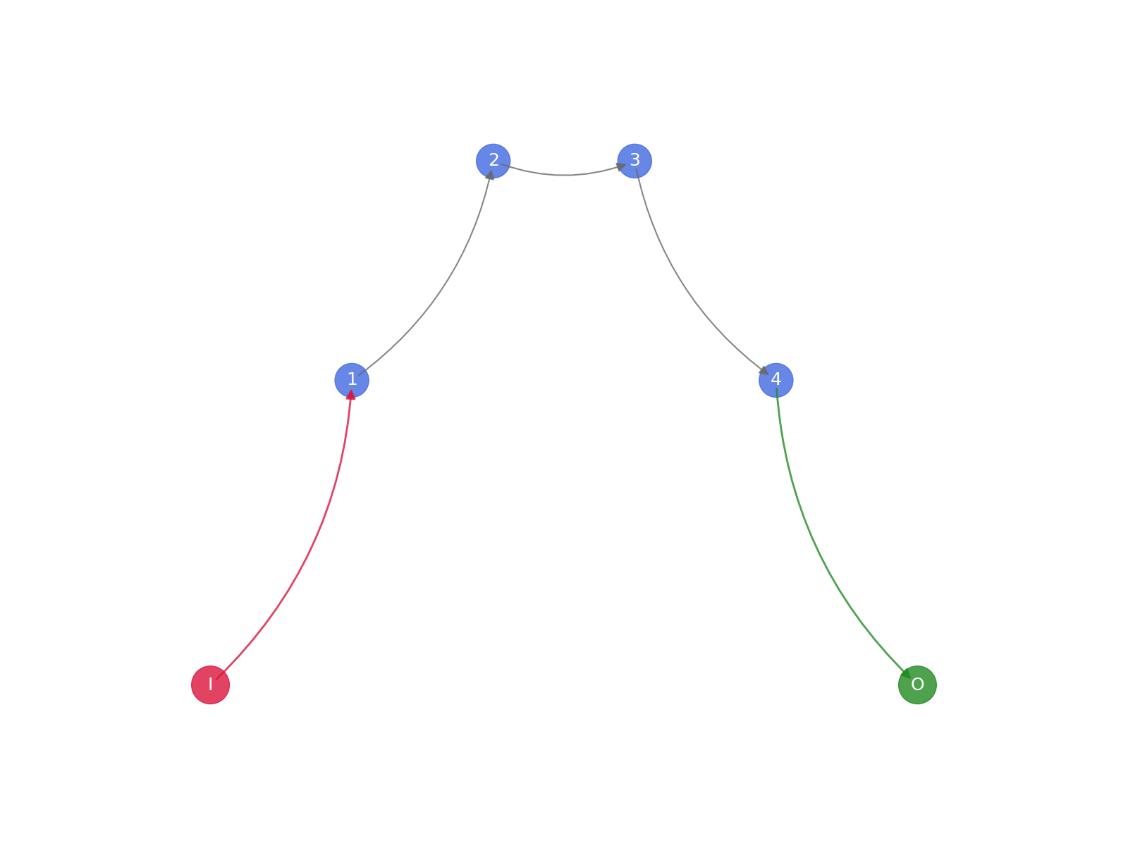
Apply the filters for step 3 and 4

task_one_data.apply_filter_sequence(
    filter_sequence=[
        SOSFrequencyFilter(sos_filter_coefficients=lowpass_filter, name="Lowpass 20"),
        ApplyFunctionFilter(
            function=lambda x: np.sqrt(np.mean(np.square(x), axis=-1)),
            is_output=True,
            name="RMS on Lowpass 20",
        ),
    ],
    representation_to_filter="Bandpass 50",
)

print(task_one_data)

task_one_data.plot_graph()

--
EMGData
Sampling frequency: 2044 Hz
(0) Input (320, 20440)

Filter(s):
(1 | 1) ChunkizeDataFilter (317, 320, 192)
(2 | 1 -> 2) Bandpass 50 (317, 320, 192)
(3 | 1 -> 2 -> 3) Lowpass 20 (317, 320, 192)
(4 | 1 -> 2 -> 3 -> 4) (Output) RMS on Lowpass 20 (317, 320)
--

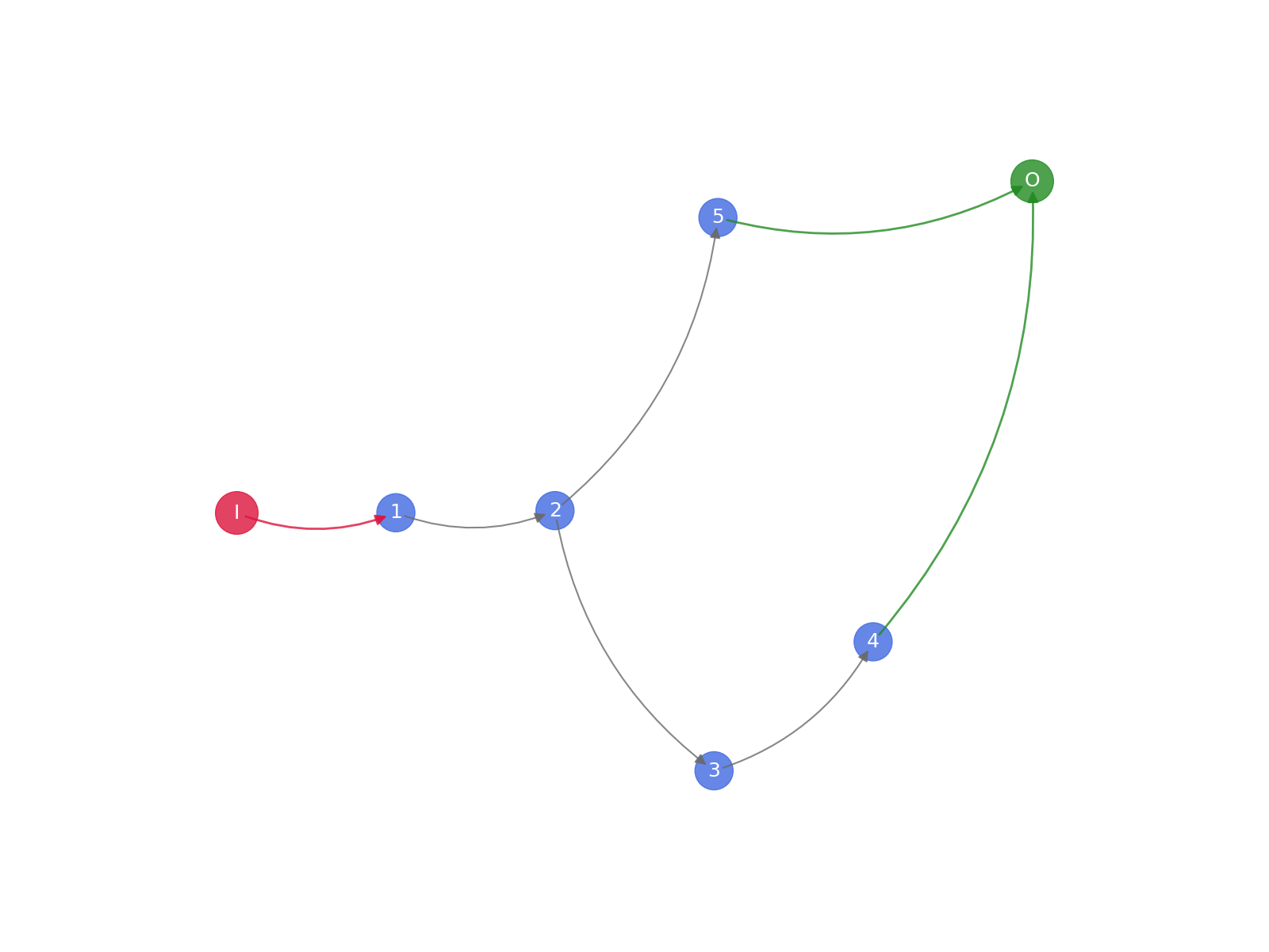
Apply the filters for step 5

task_one_data.apply_filter(
    ApplyFunctionFilter(
        function=lambda x: np.sqrt(np.mean(np.square(x), axis=-1)),
        is_output=True,
        name="RMS on Bandpass 50",
    ),
    representation_to_filter="Bandpass 50",
)

print(task_one_data)

task_one_data.plot_graph()

--
EMGData
Sampling frequency: 2044 Hz
(0) Input (320, 20440)

Filter(s):
(1 | 1) ChunkizeDataFilter (317, 320, 192)
(2 | 1 -> 2) Bandpass 50 (317, 320, 192)
(3 | 1 -> 2 -> 3) Lowpass 20 (317, 320, 192)
(4 | 1 -> 2 -> 3 -> 4) (Output) RMS on Lowpass 20 (317, 320)
(5 | 1 -> 2 -> 5) (Output) RMS on Bandpass 50 (317, 320)
--

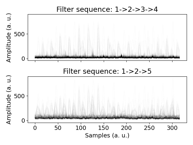
Displaying the output

import matplotlib.pyplot as plt

plt.rcParams.update({"font.size": 14})

filter_sequences = {0: "1->2->3->4", 1: "1->2->5"}

# make 2 subplots
fig, axs = plt.subplots(2, sharex=True, sharey=True)

for i, (key, value) in enumerate(task_one_data.output_representations.items()):
    for channel in range(value.shape[-1]):
        axs[i].plot(value[:, channel], color="black", alpha=0.01)

    axs[i].set_title(f"Filter sequence: {filter_sequences[i]}")
    axs[i].set_ylabel("Amplitude (a. u.)")

plt.xlabel("Samples (a. u.)")

plt.tight_layout()
plt.show()

Easier way of applying the filter pipeline

This can be achieved in a more concise way by using the apply_filter_pipeline method.

To reduce memory usage, we can set the keep_individual_filter_steps flag to False. This will remove the intermediate representations (shown in grey) from the dataset object.

Note

If new filters rely on the intermediate representations, they will be recalculated which can be computationally expensive.

task_one_data = copy(emg_data["1"])

print(task_one_data)

# Apply the filters
task_one_data.apply_filter_pipeline(
    filter_pipeline=[
        [
            ChunkizeDataFilter(chunk_size=192, chunk_shift=64),
            SOSFrequencyFilter(
                sos_filter_coefficients=bandpass_filter, name="Bandpass 50"
            ),
            SOSFrequencyFilter(
                sos_filter_coefficients=lowpass_filter, name="Lowpass 20"
            ),
            ApplyFunctionFilter(
                function=lambda x: np.sqrt(np.mean(np.square(x), axis=-1)),
                is_output=True,
                name="RMS on Lowpass 20",
            ),
        ],
        [
            ApplyFunctionFilter(
                function=lambda x: np.sqrt(np.mean(np.square(x), axis=-1)),
                is_output=True,
                name="RMS on Bandpass 50",
            )
        ],
    ],
    representations_to_filter=["Input", "Bandpass 50"],
    keep_individual_filter_steps=False,
)

print(task_one_data)

task_one_data.plot_graph()

--
EMGData
Sampling frequency: 2044 Hz
(0) Input (320, 20440)
--
Recomputing representation "Bandpass 50"
--
EMGData
Sampling frequency: 2044 Hz
(0) Input (320, 20440)

Filter(s):
(1 | 1) ChunkizeDataFilter (317, 320, 192)
(2 | 1 -> 2) Bandpass 50 (317, 320, 192)
(3 | 1 -> 2 -> 3) Lowpass 20 (317, 320, 192)
(4 | 1 -> 2 -> 3 -> 4) (Output) RMS on Lowpass 20 (317, 320)
(5 | 1 -> 2 -> 5) (Output) RMS on Bandpass 50 (317, 320)
--

Estimated memory usage: 1780 MB