Package basics

This example is a brief introduction to the basic functionalities of the package.

Loading data

First we load the EMG example data and convert it to a MyoVerse Data object. The Data object is the primary component of the package, designed to store data and apply filters. The only required parameter is the sampling frequency of the data and the data itself.

import pickle as pkl
from myoverse.datatypes import EMGData

with open("data/emg.pkl", "rb") as f:
    emg_data =  {k: EMGData(v, sampling_frequency=2044) for k, v in pkl.load(f).items()}

print(emg_data)

{'1': EMGData; Sampling frequency: 2044 Hz; (0) Input (320, 20440), '2': EMGData; Sampling frequency: 2044 Hz; (0) Input (320, 20440)}

Looking at one specific task for simplicity

The example data contains EMG from two different tasks labeled as “1” and “2”. In the following we will only look at task 1 to explain the filtering functionalities.

task_one_data = emg_data["1"]

print(task_one_data)

--
EMGData
Sampling frequency: 2044 Hz
(0) Input (320, 20440)
--

Understanding the saving format

The EMGData object has an input_data attribute that stores the raw data.

The raw data is also added to the processed_representations attribute with the key “Input”. The processed_representations attribute is a dictionary where all filtering sequences are stored. At the beginning this dictionary contains only the raw data.

The attribute is_chunked is a dictionary that stores if the data of a particular representation is chunked or not.

The attribute output_representations is a dictionary that stores the representation that will be outputted by the dataset pipeline.

print(task_one_data.input_data)

[[  53   63   74 ... -160 -173 -116]
 [ -20   -8   12 ... -194 -198 -128]
 [ -17   -4   14 ... -180 -187 -116]
 ...
 [ -89 -100 -133 ... -200 -234 -212]
 [ -27  -25  -53 ... -156 -203 -210]
 [ -11   -7  -27 ... -143 -200 -216]]

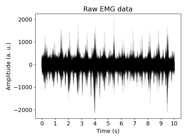
Plotting the raw data

We can plot the raw data using matplotlib.

import matplotlib.pyplot as plt
import numpy as np

raw_emg = task_one_data.input_data

# set plt font size
plt.rcParams.update({"font.size": 14})

for channel in range(raw_emg.shape[0]):
    plt.plot(raw_emg[channel], color="black", alpha=0.1)

plt.title("Raw EMG data")
plt.ylabel("Amplitude (a. u.)")
plt.xticks(
    np.arange(0, raw_emg.shape[-1] + 1, 2044).astype(int),
    np.arange(0, raw_emg.shape[-1] / 2044 + 1, 1).astype(int),
)
plt.xlabel("Time (s)")

plt.tight_layout()
plt.show()

Attributes of the EMGData object

Any Data object, of which EMGData is inheriting from, posses a processed_representations attribute where filtered data will be stored.

Note

We refer to a filtered data as a representation.

At the beginning this attribute only contains the raw data with the key “Input”.

print(task_one_data.processed_representations)

{'Input': array([[  53,   63,   74, ..., -160, -173, -116],
       [ -20,   -8,   12, ..., -194, -198, -128],
       [ -17,   -4,   14, ..., -180, -187, -116],
       ...,
       [ -89, -100, -133, ..., -200, -234, -212],
       [ -27,  -25,  -53, ..., -156, -203, -210],
       [ -11,   -7,  -27, ..., -143, -200, -216]], dtype=int16)}

Applying a filter

The EMGData object has a method called apply_filter that applies a filter to the data. For example, we can apply a 4th order 20 HZ lowpass filter to the data.

from scipy.signal import butter
from myoverse.datasets.filters.temporal import SOSFrequencyFilter

sos_filter_coefficients = butter(4, 20, "lowpass", output="sos", fs=2044)

Creating the filter

Each filter has a parameter input_is_chunked that specifies if the input data is chunked or not. This must be set explicitly as some filters can only be used on either chunked or non-chunked data. Since we want to have the result of the filter as an output representation, we set the parameter is_output to True. Further having the user specify this parameter forces them to think about the data they are working with.

lowpass_filter = SOSFrequencyFilter(
    sos_filter_coefficients, is_output=True, name="Lowpass", input_is_chunked=False
)
print(lowpass_filter)

Lowpass (SOSFrequencyFilter)

Applying the filter

To apply the filter we call the apply_filter method on the EMGData object.

task_one_data.apply_filter(
    lowpass_filter, representation_to_filter="Last"
)

print(task_one_data.processed_representations)

{'Input': array([[  53,   63,   74, ..., -160, -173, -116],
       [ -20,   -8,   12, ..., -194, -198, -128],
       [ -17,   -4,   14, ..., -180, -187, -116],
       ...,
       [ -89, -100, -133, ..., -200, -234, -212],
       [ -27,  -25,  -53, ..., -156, -203, -210],
       [ -11,   -7,  -27, ..., -143, -200, -216]], dtype=int16), 'Lowpass': array([[  30.41515398,   28.55359452,   26.67929727, ...,  -21.69369799,
         -21.72851447,  -21.75680579],
       [ -45.92706148,  -45.11724327,  -44.3360931 , ...,  -31.30362556,
         -31.32936372,  -31.35041695],
       [ -43.78353654,  -42.16849119,  -40.58739862, ...,   -5.6463695 ,
          -5.66186106,   -5.67475859],
       ...,
       [-110.89048115, -104.30581101,  -97.80368913, ...,  -15.93949333,
         -15.93448988,  -15.93147574],
       [ -56.62476067,  -49.13379821,  -41.74402497, ...,   42.30042609,
          42.27745456,   42.25766496],
       [ -39.179818  ,  -32.0000522 ,  -24.91885117, ...,   51.63322883,
          51.606299  ,   51.58321195]])}

Accessing the filtered data

The filtered data is saved in the output_representations and the processed_representations attributes of the EMGData object. In our example the key is “Lowpass”.

In case you do not want to index using the filter sequence name, you can retrieve the last processed data by indexing with “Last”.

print(task_one_data)

print(
    np.allclose(
        task_one_data.output_representations["Lowpass"],
        task_one_data["Last"],
    )
)

--
EMGData
Sampling frequency: 2044 Hz
(0) Input (320, 20440)

Filter(s):
(1 | 1) (Output) Lowpass (320, 20440)
--
True

Estimated memory usage: 973 MB