Applying Spatial Filters to EMG Data

This example demonstrates how to use spatial filters on EMG data using MyoVerse. Spatial filters operate on electrode grids to compute spatial derivatives and enhance local patterns while reducing common-mode noise.

All transforms use PyTorch tensors for CPU/GPU acceleration.

import pickle as pkl
from pathlib import Path

import matplotlib.pyplot as plt
import numpy as np
import torch

import myoverse
from myoverse.transforms import NDD, LSD, TSD, IB2, Compose, RMS, Bandpass

plt.style.use("fivethirtyeight")
plt.rcParams["axes.grid"] = False

Loading EMG Data

Load EMG data and create a tensor with grid layouts.

# Get the path to the data file
# Find data directory relative to myoverse package (works in all contexts)
_pkg_dir = Path(myoverse.__file__).parent.parent
DATA_DIR = _pkg_dir / "examples" / "data"
if not DATA_DIR.exists():
    DATA_DIR = Path.cwd() / "examples" / "data"

with open(DATA_DIR / "emg.pkl", "rb") as f:
    raw_data = pkl.load(f)["1"][:80]  # 80 channels: 64 (8x8) + 16 (4x4)

SAMPLING_FREQ = 2048

# Create grid layouts
grid1 = np.arange(64).reshape(8, 8)  # 8x8 grid
grid2 = np.arange(64, 80).reshape(4, 4)  # 4x4 grid

# Create EMG tensor with grid layouts
emg = myoverse.emg_tensor(
    raw_data,
    grid_layouts=[grid1, grid2],
    fs=SAMPLING_FREQ,
)

print(f"EMG data: {emg.names} {emg.shape}")
print(f"Grid 1: {grid1.shape}, Grid 2: {grid2.shape}")

EMG data: ('channel', 'time') torch.Size([80, 20440])
Grid 1: (8, 8), Grid 2: (4, 4)

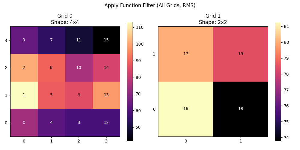
Helper function to visualize grid data

def plot_spatial_filter(emg_filtered, grid_layouts, title):
    """Plot RMS of filtered EMG on grids (normalized per grid)."""
    # Remove names for numpy conversion
    data = emg_filtered.rename(None).numpy()

    # Compute RMS over time
    rms = np.sqrt(np.mean(data**2, axis=-1))

    n_grids = len(grid_layouts)
    fig, axes = plt.subplots(1, n_grids, figsize=(5 * n_grids, 5))
    if n_grids == 1:
        axes = [axes]

    channel_offset = 0
    for i, grid_layout in enumerate(grid_layouts):
        rows, cols = grid_layout.shape
        n_channels = np.sum(grid_layout >= 0)

        # Get RMS for this grid
        grid_rms = rms[channel_offset : channel_offset + n_channels]

        # Create grid for plotting
        plot_grid = np.full((rows, cols), np.nan)
        ch_idx = 0
        for r in range(rows):
            for c in range(cols):
                if grid_layout[r, c] >= 0:
                    plot_grid[r, c] = grid_rms[ch_idx]
                    ch_idx += 1

        # Normalize per grid
        vmin = np.nanmin(plot_grid)
        vmax = np.nanmax(plot_grid)

        im = axes[i].imshow(
            plot_grid,
            cmap="rainbow",
            vmin=vmin,
            vmax=vmax,
            origin="lower",
            interpolation="nearest",
        )
        axes[i].set_title(f"Grid {i + 1} ({rows}x{cols})")
        plt.colorbar(im, ax=axes[i])

        # Add channel numbers
        ch_idx = 0
        for r in range(rows):
            for c in range(cols):
                if grid_layout[r, c] >= 0:
                    axes[i].text(
                        c, r, str(channel_offset + ch_idx),
                        ha="center", va="center", color="black", fontsize=8
                    )
                    ch_idx += 1

        channel_offset += n_channels

    fig.suptitle(title, fontsize=14)
    plt.tight_layout()
    plt.show()

Normal Double Differential (NDD) Filter

The NDD filter (Laplacian) computes differences between adjacent electrodes in a cross pattern. It enhances local spatial patterns and reduces common noise.

ndd = NDD(grids="all")
emg_ndd = ndd(emg)

print(f"NDD output: {emg_ndd.names} {emg_ndd.shape}")
plot_spatial_filter(emg_ndd, [grid1, grid2], "NDD Filter (Laplacian) - All Grids")

NDD output: ('channel', 'time') torch.Size([80, 20440])

Longitudinal Single Differential (LSD) Filter

The LSD filter computes vertical differences between adjacent electrodes.

lsd = LSD(grids="all")
emg_lsd = lsd(emg)

print(f"LSD output: {emg_lsd.names} {emg_lsd.shape}")
plot_spatial_filter(emg_lsd, [grid1, grid2], "LSD Filter (Vertical Diff) - All Grids")

LSD output: ('channel', 'time') torch.Size([80, 20440])

Transverse Single Differential (TSD) Filter

The TSD filter computes horizontal differences between adjacent electrodes.

tsd = TSD(grids="all")
emg_tsd = tsd(emg)

print(f"TSD output: {emg_tsd.names} {emg_tsd.shape}")
plot_spatial_filter(emg_tsd, [grid1, grid2], "TSD Filter (Horizontal Diff) - All Grids")

TSD output: ('channel', 'time') torch.Size([80, 20440])

Inverse Binomial 2nd Order (IB2) Filter

The IB2 filter applies a more complex spatial weighting to enhance local patterns.

ib2 = IB2(grids="all")
emg_ib2 = ib2(emg)

print(f"IB2 output: {emg_ib2.names} {emg_ib2.shape}")
plot_spatial_filter(emg_ib2, [grid1, grid2], "IB2 Filter - All Grids")

IB2 output: ('channel', 'time') torch.Size([80, 20440])

Combining Spatial and Temporal Filters

Spatial filters can be combined with temporal filters in a pipeline.

from myoverse.transforms import Stack

# Compose: Bandpass -> NDD -> RMS
pipeline = Compose([
    Bandpass(20, 450, fs=SAMPLING_FREQ, dim="time"),
    NDD(grids="all"),
    RMS(window_size=200, dim="time"),
])

output = pipeline(emg)
print(f"\nCompose output: {output.names} {output.shape}")

Compose output: ('channel', 'time') torch.Size([80, 102])

Multi-representation pipeline

Create both raw and spatially filtered representations.

# Stack creates multiple representations
multi_pipeline = Compose([
    Bandpass(20, 450, fs=SAMPLING_FREQ, dim="time"),
    Stack({
        "raw": RMS(window_size=200, dim="time"),
        "ndd": Compose([NDD(grids="all"), RMS(window_size=200, dim="time")]),
    }, dim="representation"),
])

multi_output = multi_pipeline(emg)
print(f"Multi-representation output: {multi_output.names} {multi_output.shape}")

Multi-representation output: ('representation', 'channel', 'time') torch.Size([2, 80, 102])

Visualizing Compose Output

fig, axes = plt.subplots(2, 1, figsize=(12, 8))

# Plot raw RMS
data = multi_output.rename(None).numpy()
raw_rms = data[0]  # First representation (raw)
axes[0].imshow(raw_rms, aspect="auto", cmap="rainbow")
axes[0].set_title("Raw EMG - RMS over time")
axes[0].set_ylabel("Channel")

# Plot NDD RMS
ndd_rms = data[1]  # Second representation (ndd)
axes[1].imshow(ndd_rms, aspect="auto", cmap="rainbow")
axes[1].set_title("NDD Filtered EMG - RMS over time")
axes[1].set_xlabel("Time (windows)")
axes[1].set_ylabel("Channel")

plt.tight_layout()
plt.show()

GPU Acceleration

Move to GPU for faster processing.

if torch.cuda.is_available():
    emg_gpu = emg.cuda()
    print(f"EMG on GPU: {emg_gpu.device}")

    # Apply spatial filter on GPU
    emg_ndd_gpu = ndd(emg_gpu)
    print(f"NDD on GPU: {emg_ndd_gpu.device}")
else:
    print("CUDA not available - using CPU")

CUDA not available - using CPU

Summary

Spatial filters available:

• NDD - Normal Double Differential (Laplacian)

• LSD - Longitudinal Single Differential (vertical)

• TSD - Transverse Single Differential (horizontal)

• IB2 - Inverse Binomial 2nd order

• SpatialFilter - Custom kernels

Key points:

1. Create EMG data with myoverse.emg_tensor(data, grid_layouts=[...])

2. Grid layouts are stored as tensor attributes

3. Spatial filters read grid info automatically

4. Combine with temporal filters using Compose

5. Works on both CPU and GPU

Estimated memory usage: 622 MB