Transform Basics

This example introduces the transform system - the core building block for data processing in MyoVerse. Transforms use PyTorch named tensors for dimension-aware operations that run on both CPU and GPU.

Loading Data

We load EMG data from a pickle file and wrap it as a named tensor.

import pickle as pkl
from pathlib import Path

import matplotlib.pyplot as plt
import numpy as np
import torch
import myoverse

# Get the path to the data file
# Find data directory relative to myoverse package (works in all contexts)
import myoverse
_pkg_dir = Path(myoverse.__file__).parent.parent
DATA_DIR = _pkg_dir / "examples" / "data"
if not DATA_DIR.exists():
    # Fallback for editable installs or different layouts
    DATA_DIR = Path.cwd() / "examples" / "data"

with open(DATA_DIR / "emg.pkl", "rb") as f:
    emg_data = pkl.load(f)

print("EMG data loaded successfully:")
print(f"Tasks available: {list(emg_data.keys())}")
for task, data in emg_data.items():
    print(f"\tTask '{task}': shape {data.shape}")

EMG data loaded successfully:
Tasks available: ['1', '2']
        Task '1': shape (320, 20440)
        Task '2': shape (320, 20440)

Creating Named Tensors

Named tensors have dimension names, making operations explicit. No more guessing which axis is which!

SAMPLING_FREQ = 2044

# Create named tensor with myoverse
emg = myoverse.emg_tensor(emg_data["1"], fs=SAMPLING_FREQ)

print(f"\nNamed Tensor:")
print(f"\tDimension names: {emg.names}")
print(f"\tShape: {emg.shape}")
print(f"\tDevice: {emg.device}")

Named Tensor:
        Dimension names: ('channel', 'time')
        Shape: torch.Size([320, 20440])
        Device: cpu

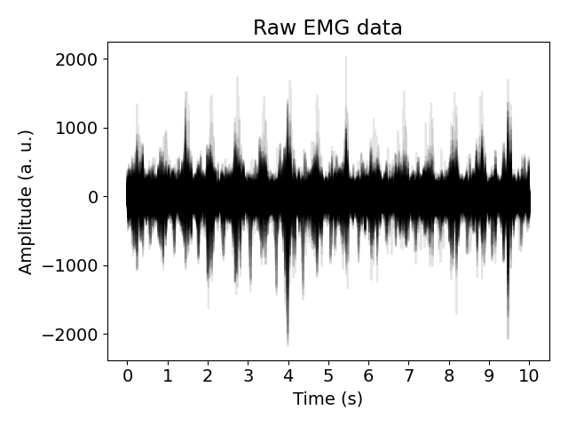
Plotting Raw Data

Visualize all channels of the raw EMG signal.

plt.style.use("fivethirtyeight")
plt.figure(figsize=(12, 6))

n_channels = emg.shape[0]
for channel in range(n_channels):
    plt.plot(emg[channel].rename(None).numpy(), color="black", alpha=0.1)

plt.title("Raw EMG Data")
plt.ylabel("Amplitude (a.u.)")
n_samples = emg.shape[1]
plt.xticks(
    np.arange(0, n_samples + 1, SAMPLING_FREQ).astype(int),
    np.arange(0, n_samples / SAMPLING_FREQ + 1, 1).astype(int),
)
plt.xlabel("Time (s)")
plt.tight_layout()
plt.show()

Dimension-Aware Transforms

Transforms explicitly specify which dimension they operate on. No more axis=-1 guessing!

from myoverse.transforms import Lowpass, Compose

# Create a lowpass filter - explicitly operates on "time" dimension
lowpass = Lowpass(cutoff=20, fs=SAMPLING_FREQ, dim="time")
print(f"\nTransform: {lowpass}")

# Apply it - dimension names are preserved!
filtered_emg = lowpass(emg)
print(f"Input names:  {emg.names}")
print(f"Output names: {filtered_emg.names}")
print(f"Dimensions are preserved!")

Transform: Lowpass(dim='time', cutoff=20, fs=2044, order=4, Q=0.707)
Input names:  ('channel', 'time')
Output names: ('channel', 'time')
Dimensions are preserved!

Compose: Chaining Transforms

Compose lets you chain multiple transforms together.

from myoverse.transforms import Highpass, Rectify

# Each transform specifies its operating dimension
feature_pipeline = Compose([
    Highpass(cutoff=20, fs=SAMPLING_FREQ, dim="time"),
    Rectify(),
])

print(f"\nCompose: {feature_pipeline}")

features = feature_pipeline(emg)
print(f"Output names: {features.names}")

Compose: Compose(
    Highpass(dim='time', cutoff=20, fs=2044, order=4, Q=0.707)
    Rectify(dim='time')
)
Output names: ('channel', 'time')

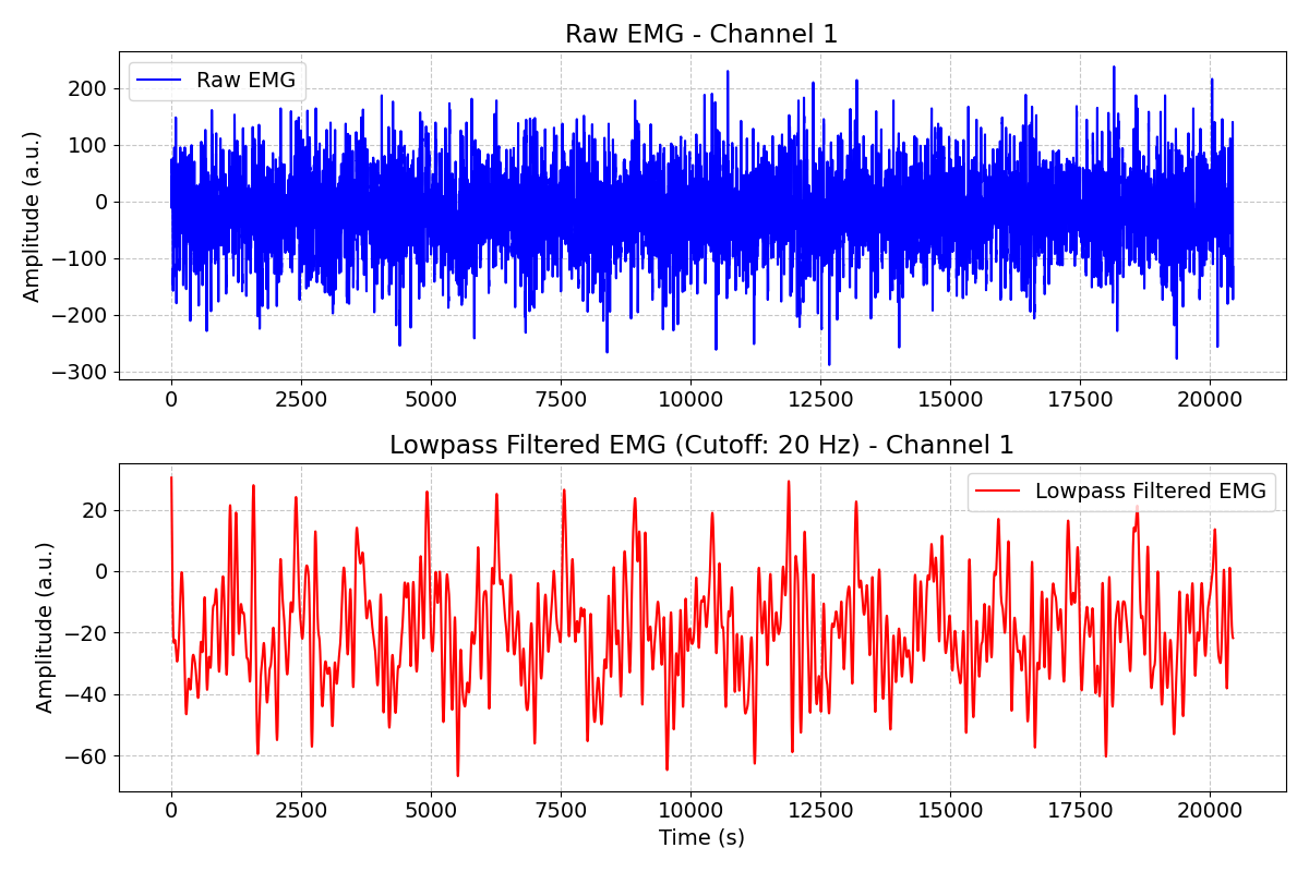
Comparing Raw vs Filtered

Let’s visualize the effect of the lowpass filter on one channel.

plt.figure(figsize=(12, 8))
channel = 0

# Raw EMG
plt.subplot(2, 1, 1)
plt.plot(emg[channel].rename(None).numpy(), label="Raw EMG")
plt.title(f"Raw EMG - Channel {channel + 1}")
plt.ylabel("Amplitude (a.u.)")
plt.legend()

# Filtered EMG
plt.subplot(2, 1, 2)
plt.plot(filtered_emg[channel].rename(None).numpy(), label="Lowpass Filtered (20 Hz)")
plt.title(f"Lowpass Filtered EMG - Channel {channel + 1}")
plt.ylabel("Amplitude (a.u.)")
plt.xlabel("Samples")
plt.legend()

plt.tight_layout()
plt.show()

Multi-Representation with Stack

Stack applies multiple transforms and combines results along a new dimension.

from myoverse.transforms import Stack, Identity

# Create raw + filtered representations
multi_repr = Stack({
    "raw": Identity(),
    "filtered": Lowpass(cutoff=20, fs=SAMPLING_FREQ, dim="time"),
}, dim="representation")

# Apply - returns stacked tensor with new dimension!
stacked = multi_repr(emg)
print(f"\nStack output:")
print(f"\tNames: {stacked.names}")
print(f"\tShape: {stacked.shape}")
print("\t(representation=2, channel, time)")

Stack output:
        Names: ('representation', 'channel', 'time')
        Shape: torch.Size([2, 320, 20440])
        (representation=2, channel, time)

Complete Pipeline: Stack in Compose

Combine Stack in a Compose for a clean workflow.

dual_representation = Compose([
    Stack({
        "raw": Identity(),
        "filtered": Lowpass(cutoff=20, fs=SAMPLING_FREQ, dim="time"),
    }, dim="representation"),
])

output = dual_representation(emg)
print(f"\nDual representation pipeline:")
print(f"\tInput:  {emg.names} {emg.shape}")
print(f"\tOutput: {output.names} {output.shape}")

Dual representation pipeline:
        Input:  ('channel', 'time') torch.Size([320, 20440])
        Output: ('representation', 'channel', 'time') torch.Size([2, 320, 20440])

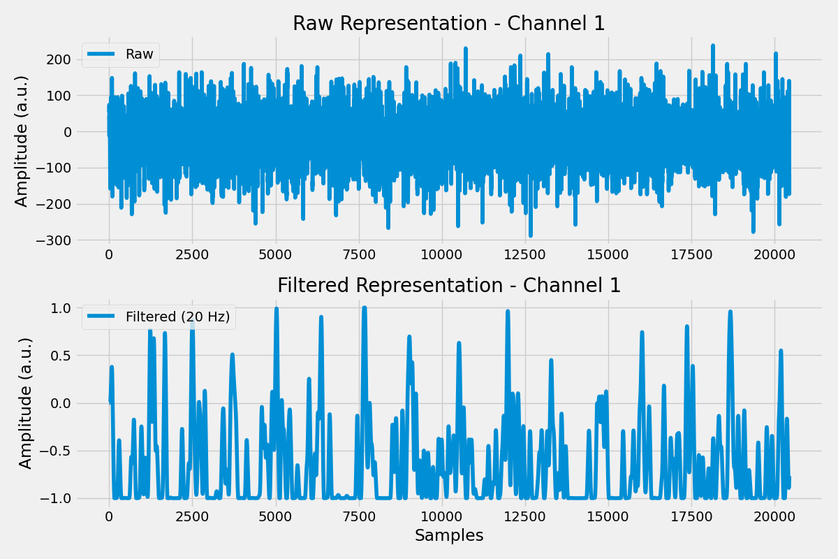
Visualizing Dual Representation

Plot both representations for one channel.

plt.figure(figsize=(12, 8))
channel = 0

plt.subplot(2, 1, 1)
plt.plot(output[0, channel].rename(None).numpy(), label="Raw")
plt.title(f"Raw Representation - Channel {channel + 1}")
plt.ylabel("Amplitude (a.u.)")
plt.legend()

plt.subplot(2, 1, 2)
plt.plot(output[1, channel].rename(None).numpy(), label="Filtered (20 Hz)")
plt.title(f"Filtered Representation - Channel {channel + 1}")
plt.ylabel("Amplitude (a.u.)")
plt.xlabel("Samples")
plt.legend()

plt.tight_layout()
plt.show()

Other Useful Transforms

MyoVerse includes many transforms for signal processing.

from myoverse.transforms import Index, Mean, ZScore

# Index: select specific elements by dimension name
select_channels = Index(indices=slice(0, 64), dim="channel")
subset = select_channels(emg)
print(f"\nIndex (first 64 channels): {emg.names}{tuple(emg.shape)} -> {subset.names}{tuple(subset.shape)}")

# Mean: average over a dimension
mean = Mean(dim="time")
averaged = mean(emg)
print(f"Mean over time: {emg.names}{tuple(emg.shape)} -> {averaged.names}{tuple(averaged.shape)}")

# ZScore: normalize over a dimension
zscore = ZScore(dim="time")
normalized = zscore(emg)
norm_data = normalized.rename(None)
print(f"ZScore: mean={float(norm_data.mean()):.6f}, std={float(norm_data.std()):.6f}")

Index (first 64 channels): ('channel', 'time')(320, 20440) -> ('channel', 'time')(64, 20440)
Mean over time: ('channel', 'time')(320, 20440) -> ('channel',)(320,)
ZScore: mean=0.000000, std=0.999976

GPU Acceleration

Move to GPU for faster processing.

if torch.cuda.is_available():
    emg_gpu = emg.cuda()
    print(f"\nEMG on GPU: {emg_gpu.device}")

    # All transforms work on GPU
    filtered_gpu = lowpass(emg_gpu)
    print(f"Filtered on GPU: {filtered_gpu.device}")
else:
    print("\nCUDA not available - using CPU")

CUDA not available - using CPU

Summary

Key concepts:

1. Named Tensors - Dimension names via myoverse.emg_tensor()

2. Transforms - Dimension-aware: Lowpass(cutoff=20, fs=2048, dim=”time”)

3. Compose - Chain transforms together (from torchvision)

4. Stack - Create multiple representations along new dimension

Benefits of dimension-aware transforms: - Self-documenting: dim=”time” vs axis=-1 - Safe: won’t accidentally filter along wrong axis - Composable: dimensions are preserved through pipelines - Fast: runs on CPU or GPU

Estimated memory usage: 1470 MB